A Recommendation Mechanism of Selecting Machine Learning Models

for Fault Diagnosis

Wen-Lin Sun

, Yu-Lun Huang

and Kai-Wei Yeh

Department of Electronics and Electrical Engineering, National Yang Ming Chiao Tung University, Hsinchu City, Taiwan,

Republic of China

Keywords:

Smart Manufacturing, Industry Automation, Fault Diagnosis, Machine Learning.

Abstract:

Faults of a machine tool generally lead to a suspension of a production line when the defeated parts need

a long lead time. The prevention of such suspension depends on the health condition of machine tools in

a factory. Hence, monitoring the health conditions of machine tools with modern Machine Learning (ML)

technologies is one of the highlights of industry evolution 4.0. Though researchers presented several methods

and mechanisms to solve the fault detection and prediction of machine tools, the current works usually focus

on deploying one ML algorithm to one speciﬁc machine tool and generating a well-trained model for fault

diagnosis and detection for that machine tool, which are impractical since a factory typically runs a variety

of machine tools. This paper presents an Automatic Fault Diagnosis Mechanism (AFDM), taking historical

data provided by an administrator and then recommending a machine-learning algorithm for fault diagnosis.

AFDM can handle different types of data, diagnose faults for different machine tools, and provide a friendly

interface for a factory administrator to select a proper analytical model for the speciﬁed type of machine tools.

We design a series of experiments to prove the diversity, feasibility, and stability of AFDM.

1 INTRODUCTION

Industry Evolution 4.0 promises new potential by in-

tegrating modern technologies with machine tools, in-

cluding the Internet of Things (IoT), cyber-physical

systems, and cloud computing. Such potential brings

the trend of smart manufacturing. The concept of

smart manufacturing innovates the existing manufac-

turing processes and achieves more intelligent fea-

tures and applications. One of the smart manufac-

turing applications is intelligent maintenance of ma-

chine tools (Kumar and Galar, 2018). After long-

term operations, the fatigue of machine components

is inevitable, which may reduce the production qual-

ity. Administrators need to stop the production lines

while waiting for the defeated components, which de-

creases the throughput of production lines. Thus, it

is crucial to monitor the health conditions of machine

tools and diagnose faults in advance.

Recently, a standard solution has been to use an

ML model to diagnose the faults of the target machine

tools. For example, FANUC, one of the largest man-

https://orcid.org/0000-0003-4298-037X

https://orcid.org/0000-0001-7618-0114

https://orcid.org/0000-0001-6262-2137

ufacturers of factory automation systems, has pre-

sented a novel service for monitoring the health con-

ditions of spindles in Computer Numerical Control

(CNC). This service ﬁrst collects the historical data

(e.g., torque values) from spindles and then trains

the ML model for predicting the anomaly score of

spindles. This service calculates the anomaly score

based on measured data during online monitoring

and warns the administrator if the score exceeds a

threshold speciﬁed by the administrator. Besides, re-

searchers have leveraged different ML models for var-

ious machine components, such as gearbox (Jia et al.,

2016), centrifugal pump (Wen et al., 2017), and drill

bit (Thirukovalluru et al., 2016). These solutions

work well but are only dedicated to speciﬁc machines

and thus may not be practical enough since most fac-

tories run more than one type of machine tool for

production. Thus a factory administrator may need a

generic fault diagnosis mechanism with a proper ML

model to develop smart factories with various ma-

chines. Moreover, most of the above solutions con-

sider accuracy the only criterion for selecting the ML

model for their machines. These solutions may skip

some essential criteria like the computation time re-

quired for generating the prediction results. The so-

Sun, W., Huang, Y. and Yeh, K.

A Recommendation Mechanism of Selecting Machine Learning Models for Fault Diagnosis.

DOI: 10.5220/0011287000003271

In Proceedings of the 19th International Conference on Informatics in Control, Automation and Robotics (ICINCO 2022), pages 49-57

ISBN: 978-989-758-585-2; ISSN: 2184-2809

lutions may not be suitable for the environment or a

speciﬁc service without careful consideration. For ex-

ample, a model generating an accurate prediction may

require a long computation time. The model may not

be suitable for a production line requiring real-time

analysis.

Factory administrators need a mechanism to rec-

ommend the best-ﬁt model according to their prefer-

ences and the production requirements. The mecha-

nism should address the above issues: (1) selecting

the best-ﬁt model for a machine tool to monitor its

health conditions; and (2) considering multiple crite-

ria when selecting the best-ﬁt model.

Hence, we propose a mechanism, AFDM, to auto-

matically recommend the best-ﬁt ML model accord-

ing to the historical data of the speciﬁed machine and

the preference given by the factory manufacturer.

2 RELATED WORK

ML algorithms can solve critical problems like fault

diagnosis of machine tools. During the fault diag-

nosis process, the ML algorithms train and generate

the corresponding classiﬁcation models to ﬁnd or pre-

dict potential faults from different components of ma-

chine tools (Leukel et al., 2021). Since the charac-

teristics of the data or signals collected from different

machine tools vary a lot, the most challenging part

of applying ML algorithms to the fault diagnosis is

how to get a proper algorithm for a speciﬁc machine

tool. This section reviews the research about fault di-

agnosis mechanisms of machine tools that adopt ML-

based classiﬁcation algorithms. The detailed compar-

ison between the related research and AFDM is dis-

cussed in Section 5.

Sun et al. (Sun et al., 2017) presented a bear-

ing fault diagnosis method based on compressed

sensing (Donoho, 2006) and deep learning. They

presented an intelligent diagnosis system with two

steps, data preprocessing and fault classiﬁcation. For

data preprocessing, they used compressed sensing

data to perform dimension reduction. They used a

Stacked Sparse Autoencoder (SSAE) with Softmax

function as the classiﬁcation model for fault classiﬁ-

cation. They tried different model parameters, includ-

ing compression ratio, number of neurons, sparsity

parameter, and decay parameter, to verify the impacts

on performance by these parameters. They compared

their work with Support Vector Machine (SVM) and

Multi-layer Perceptron (MLP) by classiﬁcation accu-

racy. Sun’s work is typical research using one algo-

rithm for one speciﬁc type of machine tool.

Selecting a proper algorithm (model) for a speciﬁc

machine tool is challenging. Brecher et al. (Brecher

et al., 2017) presented a strategy for training sev-

eral ML models (e.g., SVMs, k-Nearest Neighbors,

k-Means) with different data features to determine

which combination had the best classiﬁcation accu-

racy for a speciﬁc machine tool. In this work, the

authors estimated the state of a packing machine and

monitored the health condition of the belts of the

packing machine to predict faults in advance. These

actions could reduce unplanned downtime. Brecher’s

work showed that using different classiﬁcation mod-

els could obtain different accuracies. They selected

a model for deployment based on accuracy. How-

ever, the authors did not explain how to select a model

when encountering multiple criteria during the selec-

tion.

In 2016, Thirukovalluru et al. (Thirukovalluru

et al., 2016) presented a fault diagnosis approach en-

abled by Deep Neural Network (DNN). The work

aimed to analyze the difference in the performance

of a classiﬁcation model when using the standard fea-

tures and the features generated by DNN. The authors

ran DNN with SVM and Random Forest. Thirukoval-

luru’s approach assessed the performance of classiﬁ-

cation models by their accuracies. The results proved

that a model could improve the classiﬁcation accu-

racy with the features generated by DNN, especially

for the drilling bits. The results also showed that one

single model could not work well for all types of ma-

chine tools.

In summary, all the mentioned works performed

data preprocessing when dealing with signals from

machine tools, deployed ML algorithms to classify

the processed data, and selected a suitable model

based on the classiﬁcation accuracy. However, none

of them has considered the multiple types of machine

tools and the multiple criteria for model selection. To

address these two issues, we generalize these meth-

ods and propose AFDM in Section 3. AFDM adopts

multiple ML algorithms for multiple types of machine

tools. AFDM trains, evaluates and ranks the models

for a speciﬁed machine tool when considering multi-

ple criteria.

3 AFDM

By leveraging modern ML algorithms, smart facto-

ries can predict machine faults in advance, increase

the production line’s throughput, and reduce manu-

facturing costs. We propose AFDM, an Automatic

Fault Diagnosis Mechanism, for selecting the best-ﬁt

classiﬁcation model to diagnose and predict faults for

different machine tools and help the factories build

ICINCO 2022 - 19th International Conference on Informatics in Control, Automation and Robotics

up an intelligent manufacturing system. By adopting

multiple-criteria decision-making (MCDM) methods

to AFDM, we can recommend better-ﬁt classiﬁca-

tion models according to the characteristics of the

collected data and the customized requirements (e.g.,

limited training time) to diagnose faults of machine

tools.

3.1 Overview

AFDM provides an objective way to help factory

administrators get more insights into their machine

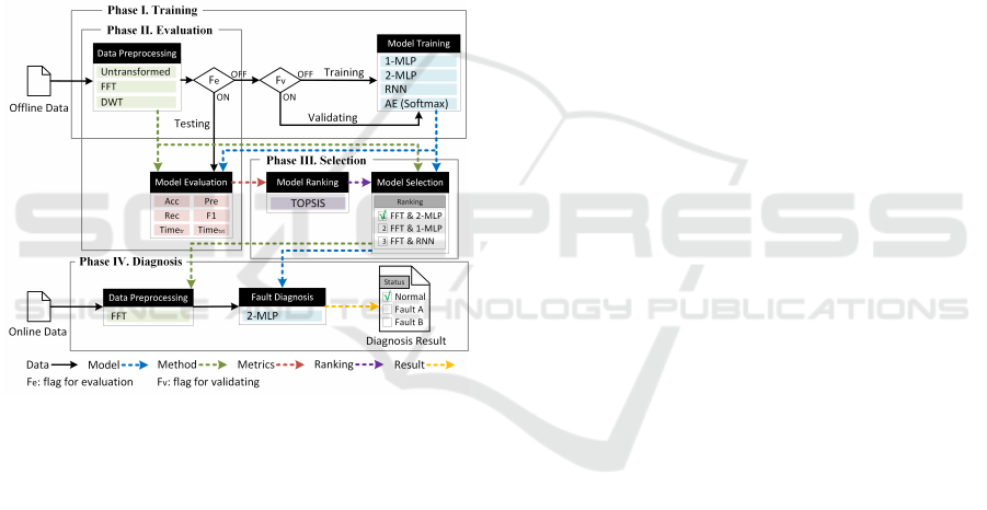
tools. Figure 1 illustrates the fault diagnosis proce-

dure of AFDM and its implementation. The proce-

dure contains four phases, including Training, Evalu-

ation, Selection, and Diagnosis (Phase I to IV in Fig-

ure 1, respectively).

Figure 1: The Fault Diagnosis Procedure of AFDM.

By reviewing the existing literature, we can ﬁnd a

general fault diagnosis procedure that includes model

training and fault diagnosis. Generally, the existing

methods train a classiﬁcation model with ofﬂine data.

Then, the trained model is deployed to a ﬁeld and

analyzes the online data in the fault diagnosis phase.

AFDM revises the traditional procedure and adds two

more phases (Evaluation and Selection) for an auto-

matic recommendation.

Different from other methods, AFDM trains mul-

tiple classiﬁcation models with different ML algo-

rithms at a time. When an administrator launches

AFDM in a factory, the administrator collects data

from the machines in the factory. In the ﬁrst phase,

the administrator enters the collected data to AFDM

for training multiple classiﬁcation models (e.g., 1-

MLP, 2-MLP, RNN, and AE (Softmax) in Figure 1).

Phase II estimates these models’ performance (like

accuracy.) Then, according to the evaluation metrics,

AFDM ranks these models and recommends the best-

ﬁt model to the administrator in Phase III. If the ad-

ministrator accepts the recommended model, AFDM

diagnoses the data acquired from machine tools in

the factory using the model selected in the Diagno-

sis phase. The following subsections detail the four

phases.

3.2 Phase I: Training

We design the Training phase to tune classiﬁcation

models that may be candidates for the speciﬁed ma-

chine tool. In this phase, AFDM tunes the candidate

classiﬁcation models with the historical data collected

from the target machine tool. In the Training phase,

AFDM designs two primary operations for training

multiple classiﬁcation models: Data Preprocessing

and Model Training (see Figure 1). Depending on the

data type, some data cannot be analyzed in its raw

format. For example, the features of raw signals are

sometimes hard to be discovered in the time domain.

These types of data should be ﬁltered or converted be-

fore further processing. The primary purpose of Data

Preprocessing is to prepare raw data for subsequent

training. AFDM transforms the raw data into another

domain depending on the data type. For instance, FFT

is a popular preprocessing method that transforms sig-

nals (raw data) into the frequency domain and quickly

extracts and analyzes the signals’ features.

When realizing AFDM, we can install plenty of

data preprocessing methods as a plug-in, like slic-

ing the raw signals into pieces (Untransformed), FFT,

and DWT. After preprocessing, AFDM splits the pro-

cessed data into three sets: training, validation, and

testing sets. Namely, data in the training set trains the

classiﬁcation models, data in the validation set tunes

the parameters of the classiﬁcation models, and the

testing data evaluates the performance of the classi-

ﬁcation models installed in AFDM. We design two

ﬂags (F

and F

) to control the processing of train-

ing, validating, and testing. Once F

is ON, AFDM

forwards data to Model Evaluation in Phase II; oth-

erwise, AFDM forwards the data to Model Training.

Once F

is ON, data is used to validate the trained

models in Model Training; otherwise, data is used to

train the classiﬁcation models listed in Model Train-

ing.

Different classiﬁcation models function differ-

ently. Some classiﬁcation models are suitable for non-

linear data, while others are more effective when deal-

ing with time-series data. To make AFDM analyze

different data types, we install three variants of arti-

ﬁcial neural networks in AFDM as the default clas-

siﬁcation models, including MLP, Recurrent Neural

A Recommendation Mechanism of Selecting Machine Learning Models for Fault Diagnosis

Network (RNN), and Autoencoder (AE) with Soft-

max function. For simplicity, we deﬁne 1-MLP and

2-MLP for MLP with one and two hidden layers, re-

spectively. MLP is a class of feedforward neural net-

works. In addition to the input and output layers,

MLP contains some hidden layers, and neurons in two

adjacent layers are interconnected.

RNN leverages sequential information of the in-

put data from the previous step and feeds it as input to

the next step, which is beneﬁcial to recognizing pat-

terns of time series data like text and speech recog-

nition. AE learns a good representation of input data

and is suitable for dimension reduction. AE extracts

features from the input data and generates the reduced

representations that can reconstruct the original data.

An AE model contains an encoder to explore features

and a decoder to reconstruct input data. By running

with a Softmax function at the output of the encoder,

an AE model can perform data classiﬁcation.

The upper rectangle in Figure 1 shows the imple-

mentation of the Training phase. As illustrated in

the ﬁgure, the default methods for Data Preprocess-

ing are ‘untransformed,’ ‘FFT,’ and ‘DWT,’ where the

‘Untransformed’ means no preprocessing is required.

Data will be forwarded to the next phase as it is. The

default classiﬁcation models for Model Training in

Phase I include 1-MLP, 2-MLP, RNN, and AE (Soft-

max). An administrator can extend the preprocessing

methods and classiﬁcation models listed in Phase I as

needed.

3.3 Phase II: Evaluation

AFDM mainly targets ranking and recommending the

best-ﬁt classiﬁcation model to an administrator to an-

alyze and predict faults of machine tools. Based on

the results of analyzing the raw signals collected from

the machine tools in the factory, AFDM makes rec-

ommendations to the administrator. Thus, AFDM

needs to be able to handle different types of signals

provided by different types of machine tools. For this

purpose, AFDM has to evaluate different classiﬁca-

tion models’ performance (e.g., prediction accuracy)

and ﬁnd the best-ﬁt model for the speciﬁed machine

tool(s).

Then, AFDM evaluates the classiﬁcation mod-

els trained in the previous phase. The Evaluation

phase contains two signiﬁcant operations: Data Pre-

processing and Model Evaluation, as illustrated in

Figure 1. The Data Preprocessing operation in the

Training and Evaluation phases are the same. Signals

are forwarded to Model Evaluation as it is when ‘Un-

transformed’ is selected. Signals are processed and

forwarded to the next phase when ‘FFT,’ ‘DWT,’ or

other data preprocessing methods are selected. Com-

pared with other research, the Model Evaluation oper-

ation works similarly to the model testing operation in

other research. After testing the classiﬁcation models

trained in Phase I with the preprocessed data, AFDM

calculates the performance for those trained models in

terms of different metrics, including accuracy (Acc),

precision (Pre), recall (Rec), f1-score (F1), training

time (Time

), and testing time (Time

tst

) (Ali et al.,

2017; Mehdiyev et al., 2016).

The ﬁrst four metrics, Acc, Pre, Rec, and F1, are

deﬁned by the confusion matrix for a two-class clas-

siﬁcation problem. The training time Time

is the

computation time required for training and tuning a

classiﬁcation model. The testing time Time

tst

is the

computation time required for making a single pre-

diction. AFDM uses these metrics to evaluate and

rank the candidates of classiﬁcation models trained in

Phase I.

3.4 Phase III: Selection

According to the evaluation results obtained in Phase

II, AFDM can rank the classiﬁcation models trained

in Phase I. The Selection phase deﬁnes two opera-

tions: Model Ranking and Model Selection. Model

Ranking ranks the classiﬁcation models by the met-

rics deﬁned in the Evaluation phase and the pref-

erences speciﬁed by a factory administrator. Since

AFDM ranks models with multiple metrics, Phase III

deals with an MCDM problem, so we cannot simply

apply a sorting algorithm to rank these models. Some

algorithms, like Analytic Hierarchy Process (AHP),

Adjusted Ratio of Ratios (ARR), and Technique for

Order of Preference by Similarity to Ideal Solution

(TOPSIS). This research adopts TOPSIS in AFDM to

solve such an MCDM problem. Conceptually, TOP-

SIS selects a positive ideal (best) solution and a neg-

ative ideal (worst) solution for each criterion (metric)

and then ranks each candidate solution with its Rela-

tive Closeness (RC). The deﬁnition of RC is:

RC =

∗

+ S

−

,0 ≤ RC ≤ 1. (1)

The equation deﬁnes a ratio of the distance of the can-

didate to the positive ideal solution (S

∗

) and the dis-

tance to the negative ideal solution (S

−

). A higher

RC represents a better solution, which should have a

higher ranking. With TOPSIS, AFDM can rank the

classiﬁcation models and generate an ordered list of

models (ranking). After obtaining the list, the admin-

istrators can select the best-ﬁt classiﬁcation model for

their factory according to the ranking, experience, or

other considerations. The rectangle of Phase III in

ICINCO 2022 - 19th International Conference on Informatics in Control, Automation and Robotics

Figure 1 shows the processes of the Selection phase

and its implementation.

3.5 Phase IV: Fault Diagnosis

The primary purpose of the previous three phases is

to train and determine the best-ﬁt classiﬁcation model

according to the historical data collected from the ma-

chine tools. The operations are time-consuming, so

that we can process the operations in an ofﬂine man-

ner. The fourth phase, the Diagnosis phase, is a pro-

cess for diagnosing data collected from machine tools

in real-time. The diagnosis should proceed immedi-

ately.

The Diagnosis phase contains two operations:

Data Preprocessing and Fault Diagnosis. Similar to

the Data Preprocessing in Phase I and II, the Data

Preprocessing in Phase IV transforms the raw signals

into a different type of data so that AFDM can extract

features for analysis more efﬁciently. The only differ-

ence is that Data Preprocessing in the Diagnosis phase

contains only one preprocessing method according to

the classiﬁcation model selected in Phase III. After

preprocessing, we analyze the raw signals and the ex-

tracted features by the selected model. The analyzed

results (diagnosis results) present the current status of

the target machine tool. The administrator can moni-

tor the target machine tools through diagnosis results.

The Phase IV rectangle in Figure 1 shows the pro-

cesses and implementation of the Diagnosis phase.

4 EXPERIMENTS

This section conducts four experiments to investigate

the functionality of the main building blocks designed

in AFDM. The four experiments include one diver-

sity test, two feasibility tests, and one stability test.

The diversity test shows AFDM’s ability to handle

raw signals collected from different types of machine

tools (e.g., bearing, hydraulic pump, and drill bit).

Then, we use the feasibility tests to show the feasibil-

ity of each phase in AFDM. In the ﬁrst feasibility test,

we investigate the impact of different data preprocess-

ing methods with the same classiﬁcation model. We

evaluate and rank multiple classiﬁcation models using

different conﬁgurations in the second feasibility test.

Finally, in the stability test, we investigate the stability

of the ranking method (TOPSIS) adopted in AFDM.

We evaluate the ranking results of AFDM by deploy-

ing various weights of the selected performance met-

rics.

4.1 Diversity Test

As mentioned in section 3.3, one of the signiﬁcant ob-

jectives of AFDM is to recommend the best-ﬁt clas-

siﬁcation model according to the characteristics of

the input data. With so, AFDM can provide a ﬂex-

ible fault diagnosis mechanism for various machine

tools. To show AFDM’s diversity, we deploy differ-

ent types of datasets to AFDM. In this experiment,

we use datasets from different institutions with dif-

ferent kinds of machine tools, including one from

Case Western Reserve University (CWRU) with bear-

ing (Bearing 1), one from the University of Cincinnati

with bearing (Bearing 2), one from Beihang Univer-

sity with hydraulic pump (Pump), and two from In-

dian Institute of Technology with drill bit (Drill 1 and

Drill 2).

We train these datasets with 2-MLP models and

list their performance metrics in Table 1. The accu-

racy of Bearing 1, Bearing 2, and Pump exceeds 0.8.

The accuracy for Drill 1 and Drill 2 falls below 0.5.

The results imply that we cannot apply a single algo-

rithm to analyze raw signals collected from different

types of machine tools. The results conclude that we

need multiple classiﬁcation models for analyzing data

of different types. A fault diagnosis mechanism needs

to select a dedicated model according to the charac-

teristics of data (raw signal) collected from a machine

under-diagnosis. If a factory administrator has no idea

which model should be selected, he or she may need

a recommendation mechanism.

Moreover, the results show the diversity of AFDM

to handle various types of data from different machine

tools. For simplicity, we use the CWRU dataset in the

subsequent experiments.

4.2 Feasibility Test I: Different Data

Preprocessing Methods

In this experiment, we evaluate the inﬂuences of dif-

ferent data preprocessing methods based on the per-

formance of a classiﬁcation model. In Phase I, we

choose 2-MLP as the classiﬁcation model, and each

hidden layer contains 100 neurons. Then, we train the

classiﬁcation models with the same dataset, split ratio,

and hyper-parameter but using different data prepro-

cessing methods. We split the dataset into two sub-

sets, 70% for training and 30% for testing. The train-

ing data contains the validation data.

We design six cases with different preprocessing

methods in the experiment, including one with FFT,

four with DWT, and one with untransformed. For

DWT, we adopt four different conﬁgurations, includ-

ing level 1 to 3 detail coefﬁcients and approxima-

A Recommendation Mechanism of Selecting Machine Learning Models for Fault Diagnosis

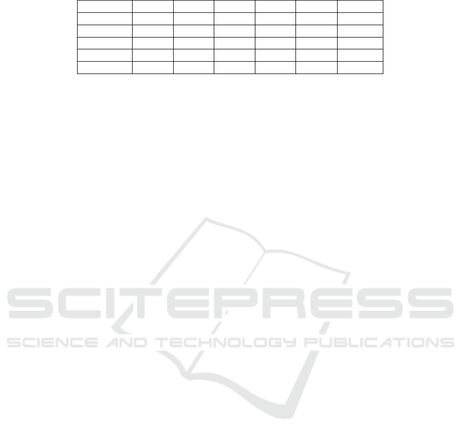
Table 1: Results of Diversity Test.

Acc Pre Rec F1 Time

Time

tst

Bearing 1 0.8389 0.8444 0.8377 0.8410 1.2319 0.00058

Bearing 2 0.8581 0.8624 0.8566 0.8595 0.8409 0.00045

Pump 0.8226 0.8569 0.8284 0.8424 0.4707 0.00049

Drill 1 0.3885 0.3751 0.3861 0.3805 0.7361 0.00054

Drill 2 0.4889 0.4883 0.4887 0.4885 5.0848 0.00058

tion coefﬁcients (abbreviated as DWT-L1, DWT-L2,

DWT-L3, and DWT-approx). We use the untrans-

formed data as the baseline for these cases. Each case

repeats ten times with different random seeds, and

then we calculate the average of each performance

metric.

Table 2 shows the prediction results obtained

when applying different data preprocessing methods

to the classiﬁcation model. The accuracy falls be-

tween 0.8394 and 1, precision falls between 0.8571

and 1, recall falls between 0.8394 and 1, and F1-score

falls between 0.8481 and 1. When applying FFT to

the raw signals, the accuracy is higher than in any

other cases using DWT. Compared with the raw sig-

nals (untransformed), most cases activating data pre-

processing have better prediction accuracy, except the

one using DWT-L3. The results show that activat-

ing data preprocessing methods may extract essential

features from the raw signals and help train the clas-

siﬁcation model. As for the computation time, four

DWT cases require less time than the untransformed

case. When applying DWT, both training time and

testing time tend to increase as the dimension of data

increases. This experiment requires more time to train

the model when using FFT.

Since data preprocessing may affect the prediction

accuracy of a classiﬁcation model, AFDM provides

the ﬂexibility to bundle a preprocessing method and

a classiﬁcation model as a pair for ranking. Addi-

tional metrics, such as the preprocessing time, may

be required when ranking such pairs. Hence, AFDM

also provides the ﬂexibility for adding these addi-

tional metrics in Phase II.

4.3 Feasibility Test II: Different

Conﬁgurations and Parameters

While model training, we can apply different con-

ﬁgurations and parameters to an ML algorithm and

generate different classiﬁcation models for better per-

formance. This experiment considers four ML algo-

rithms: 2-MLP, 1-MLP, RNN, and AE with Softmax

function. Each algorithm has a different conﬁguration

(different numbers of hidden layers and neurons). 1-

MLP and RNN have only one hidden layer, 2-MLP

has two hidden layers, and AE has four hidden layers.

We mark the conﬁguration on the superscript of each

algorithm. For example, we mark a 2-MLP algorithm

running with two hidden layers, in which each layer

has 100 neurons, as 2-MLP

(100,100)

, as illustrated in

Table 3.

Same as the previous experiment, the experiment

analyzes the CWRU dataset (bearing). The percent-

age of training data to all data is 70%, and valida-

tion data is included in the training data. In this ex-

periment, we do not activate any data preprocessing

method. Data is untransformed. The experiment re-

peats ten times with different random seeds. Then,

we calculate the average of each performance met-

ric. AFDM ranks the twelve classiﬁcation models and

recommends one of them as the best-ﬁt model. The

experiment investigates the impact of different con-

ﬁgurations.

Table 3 shows the performance metrics of the

twelve models. The results show that more neu-

rons lead to better accuracy, precision, recall, and F1-

score. Generally, more time is required to train and

test a model when using more neurons. Neverthe-

less, there might be exceptions in some cases. Even

if fewer neurons are used, a model can still get bet-

ter prediction results and a shorter training time. For

example, in 2-MLP

(100,100)

, the model has better per-

formance than 2-MLP

(10,10)

and 2-MLP

(1000,1000)

. 2-

MLP

(100,100)

has the best performance both in the pre-

diction accuracy and computational time.

Compared to the models using 1-MLP, 2-MLP,

and RNN, RNN has better prediction accuracy than

1-MLP and 2-MLP when these models use the same

number of neurons of the hidden layers. Undoubt-

edly, more time is required to train the RNN model

and make a prediction. As for AE with the Soft-

max function, the results show that AE

(1000,200,40,5)

(1500,300,60,8)

, and AE

(2000,400,80,10)

obtain similar

prediction accuracy, but the training and testing times

increase as the network grows.

Since six performance metrics are used in AFDM

to rank the twelve models, factory administrators need

to decide the relative weights of the metrics to get the

best-ﬁt model for the factory. In this experiment, we

give equal weights to the six metrics. AFDM uses

ICINCO 2022 - 19th International Conference on Informatics in Control, Automation and Robotics

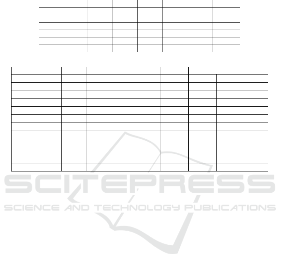
Table 2: Results of Feasibility Test I.

Acc Pre Rec F1 Time

Time

tst

FFT 1 1 1 1 3.5418 0.00039

DWT-L1 0.8880 0.9054 0.8902 0.8977 0.9355 0.00050

DWT-L2 0.8704 0.8965 0.8689 0.8824 0.7040 0.00046

DWT-L3 0.8394 0.8571 0.8394 0.8481 0.6830 0.00045

DWT-approx 0.8610 0.8748 0.8577 0.8662 0.6948 0.00044

Untransformed 0.8477 0.8568 0.8490 0.8529 1.2729 0.00055

Table 3: Results of Feasibility Test II.

Acc Pre Rec F1 Time

Time

tst

RC Rank

2-MLP

(10,10)

0.7343 0.7436 0.7388 0.7412 1.3121 0.00057 0.88080 4

2-MLP

(100,100)

0.8408 0.8480 0.8440 0.8460 1.3057 0.00057 0.95922 1

2-MLP

(1000,1000)

0.7939 0.7984 0.7937 0.7961 2.5651 0.00071 0.87845 5

1-MLP

(10)

0.7040 0.7107 0.7079 0.7093 1.3615 0.00051 0.86176 6

1-MLP

(100)

0.8197 0.8230 0.8214 0.8222 1.3756 0.00054 0.94452 2

1-MLP

(1000)

0.8328 0.8275 0.8332 0.8303 2.5778 0.00062 0.91150 3

RNN

(10)

0.7357 0.7373 0.7338 0.7356 7.3714 0.00112 0.61100 8

RNN

(100)

0.8481 0.8650 0.8470 0.8559 3.1549 0.00115 0.76070 7

RNN

(1000)

0.8829 0.8890 0.8824 0.8857 8.6092 0.00255 0.30280 12

(1000,200,40,5)

0.8767 0.8776 0.8715 0.8745 10.0747 0.00075 0.60286 9

(1500,300,60,8)

0.8702 0.8708 0.8706 0.8707 12.1400 0.00084 0.52780 10

(2000,400,80,10)

0.8757 0.8772 0.8764 0.8768 14.7346 0.00088 0.46457 11

TOPSIS for ranking the models by the six metrics.

The RC value of each model is calculated and listed

in the second last column of Table 3.

In the table, we can see that 2-MLP

(100,100)

has

the highest RC (0.95922), and 1-MLP

(100)

owns the

second-high RC value (0.94452). The RC values of

the two models are very close. Whenever there is

any vibration of evaluation results, the rank of the

models may change. The administrator can substitute

the working model with the recommended one. The

substitution between the models may cost some over-

heads. The overheads could be considerable since the

structures (e.g., the number of hidden layers and the

number of neurons in each hidden layer) vary signif-

icantly between ML algorithms. Thus, we design the

fourth experiment, the Stability Test, for further dis-

cussions about the stability of model ranking.

4.4 Stability Test: Stable Model

Ranking

AFDM recommends the best-ﬁt classiﬁcation model

for fault diagnosis by ranking the candidates with the

performance metrics. The variation of ranking may

cause model substitution. The substitution can be as

small as modifying hyper-parameters only or as big

as changing the structure of the classiﬁcation model.

If the ranking of models varies from time to time, the

substitution overhead could be considerable and inﬂu-

ence the overall performance. In this experiment, we

evaluate the stability of TOPSIS’s rankings when the

weights of performance metrics change.

To observe the weights and rankings, we only con-

sider the relative changes in weights between two per-

formance metrics: accuracy and training time. We de-

ﬁne two weights for the two metrics, the weight of ac-

curacy (w

) and the weight of training time (w

). The

summation of the two weights is 1. We choose the

top-six cases in Table 3 and evaluate the changes in

their rankings for the varied weights. w

varies from

1 to 0 and w

from 0 to 1. The combination of the

weights are recorded as w

(e.g., 0.6/0.4.) Fig-

ure 2 shows the change in rankings for the selected

models.

In TOPSIS, the ranking is generated based on

the RC value of each candidate in descending order.

Thus, a larger RC stands for a higher ranking. In

Figure 2, we can see that 2-MLP

(100,100)

has the

highest RC value (RC = 1) among all cases. AFDM

ranks the 2-layer MLP with 100 neurons in the

hidden layer as the best solution within all the com-

binations of weights. 1-MLP

(100)

(the line marked

with ⋆) is the second candidate recommended for the

cases using the weight combinations from 0.9/0.1

A Recommendation Mechanism of Selecting Machine Learning Models for Fault Diagnosis

Figure 2: RC values under different combination of

weights.

to 0.3/0.7. In short, the rankings of 2-MLP

(100,100)

and 1-MLP

(100)

remain unchanged under the weight

combinations within the range of 0.9/0.1 to 0.3/0.7.

As for other models, the rankings vary as the rel-

ative weights change. For example, when w

is con-

sidered much more important than w

, 2-MLP

(10,10)

and 1-MLP

(10)

are recommended; otherwise, AFDM

recommends 2-MLP

(1000,1000)

and 1-MLP

(1000)

. The

results show that AFDM can consider administrators’

preferences while keeping the generated rankings sta-

ble to a certain extent. This experiment proves that

adopting TOPSIS as the selection method in AFDM

can obtain feasible, adaptable, and stable results.

5 DISCUSSION

We compare AFDM with Sun’s, Brecher’s, and

Thirukovalluru’s work and summarize their differ-

ences in Table 4. As shown in Table 4, the compar-

ison contains three different aspects: target, training,

and evaluation. The target aspect indicates whether a

candidate supports fault diagnosis targeting multiple

types of machine tools. The training aspect shows the

ability to support different data preprocessing meth-

ods and ML models for fault diagnosis. The evalu-

ation aspect discloses the metrics emphasized during

model evaluation.

Sun’s work used a bearing dataset from CWRU

as the input data and identiﬁed the fault conditions

of bearings. In Brecher’s work, a packing machine

was considered, which monitored the health condi-

tions of the belt. Although Brecher et al. mentioned

the possibility of supporting multiple machines with

cloud computing technology, the detail about related

design was lacking. Thus we marked this feature as

△. Among the related work, only Thirukovalluru’s

work investigated the diagnosis for different machine

tools, including an air compressor, drill bit, bearing,

and steel plate. In this paper, we design and imple-

ment AFDM to diagnose faults of bearing, drill bit,

and pump, but the framework of AFDM is also ﬂexi-

ble in analyzing faults of different machine tools.

In Sun’s and Thirukovalluru’s works, the re-

searchers adopted one primary ML algorithm to im-

prove the model training process for the target ma-

chine tool. Differently, Sun et al. directly deployed

SSAE as the classiﬁcation model, and Thirukoval-

luru et al. applied DNN to improve the classiﬁ-

cation models through feature extraction. None of

them mentioned how to customize the data prepro-

cessing methods and classiﬁcation models such that

an administrator can analyze the data of their ma-

chine tools more precisely. In Brecher’s work, the

authors applied many ML algorithms to diagnose the

belt faults with different data features. Then, the au-

thors selected the model with the best accuracy for

their packing machine. Comparatively, AFDM pro-

vides a ﬂexible framework and allows an administra-

tor to install user-deﬁned data preprocessing meth-

ods and classiﬁcation models. An administrator can

specify the weights of performance metrics to ﬁnd

the best-ﬁt model(s) for their machine tools. Such a

design makes AFDM adaptable to different scenarios

and users’ preferences.

Most related works selected a classiﬁcation model

based on accuracy. Sun’s work investigated each clas-

siﬁcation model’s classiﬁcation accuracy and compu-

tation time. Although they considered the trade-off

between accuracy and computation time, they did not

explain how to solve it when making the ﬁnal selec-

tion. Also, they did not specify what kind of com-

putation time they used for model evaluation, so we

marked both the training and testing time as △. In

Brecher’s work, the authors investigated the advan-

tages and disadvantages of each classiﬁcation model

but did not specify how they selected the model based

on these advantages and disadvantages. Thus we

mark their support of other criteria as △.

With AFDM, an administrator can select the best-

ﬁt classiﬁcation model based on the recommended

rankings generated by TOPSIS. The administrator

only needs to determine the relative weight of each

performance metric according to their preferences

and experiences, and then AFDM can automatically

generate rankings of the classiﬁcation models. In ad-

dition to the performance metrics used in the exper-

iments, the administrator can add more quantitative

criteria for evaluating classiﬁcation models, showing

the ﬂexibility of AFDM in model selection.

ICINCO 2022 - 19th International Conference on Informatics in Control, Automation and Robotics

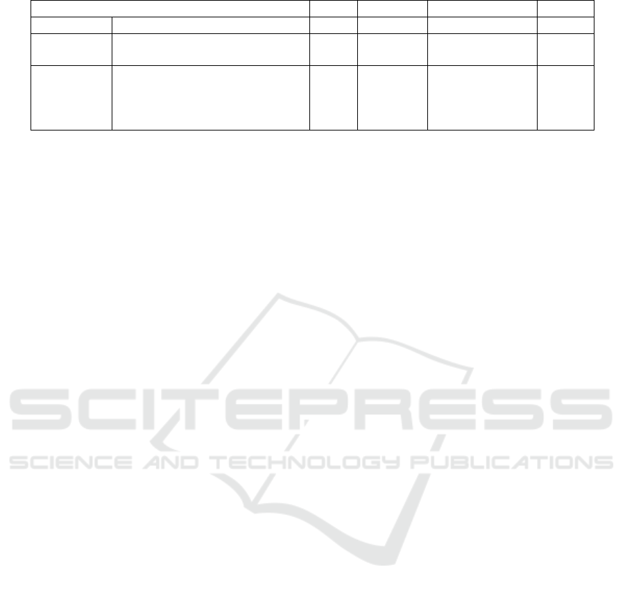
Table 4: Comparison among fault diagnosis mechanisms.

Supporting Features Sun’s Brecher’s Thirukovalluru’s AFDM

Target Multiple Machine Tools ✗ △ ✓ ✓*

Training

Multiple Preprocessing Methods ✗ ✗ ✗ ✓*

Multiple ML Models ✗ ✓ ✓ ✓*

Evaluation

Accuracy ✓ ✓ ✓ ✓

Training Time △ ✗ ✗ ✓

Testing Time △ ✗ ✗ ✓

Others ✗ △ ✗ ✓*

support customized options

6 CONCLUSION

Nowadays, rapidly developing ML technology and re-

lated applications are introduced to manufacturing to

make it “smarter.” Fault diagnosis of machine tools,

for example, traditionally depended on the experience

owned by the administrators. However, by deploy-

ing ML technology, the faults of running machine

tools can be detected or even predicted immediately.

This paper proposes AFDM, a generic fault diagnosis

mechanism for different machine tools. AFDM, op-

erating in four phases, can automatically recommend

the best-ﬁt model according to multiple metrics, in-

cluding the nature of input data and user preferences.

We conduct four experiments to show AFDM’s diver-

sity in handling various data from different machine

tools, the feasibility of conﬁguring different meth-

ods and parameters in each phase, and the stability

in ranking and recommending the best-ﬁt classiﬁca-

tion model. In comparison to existing works, AFDM

is the only approach that can:

1. adapt to various data from different kinds of ma-

chine tools,

2. support multiple data preprocessing methods and

ML models, and

3. stably evaluate and rank the candidate models

with multiple criteria, where the weight of each

criterion is conﬁgurable.

AFDM leaves ﬂexibility for administrators to add or

select data preprocessing methods, ML algorithms,

and metrics to train and evaluate the models according

to the user’s experience. We conclude that AFDM can

stably and automatically recommend the best-ﬁt ML

model for the fault diagnosis of machine tools based

on user’s preferences.

ACKNOWLEDGEMENTS

This work was ﬁnancially supported in part by Min-

istry of Science and Technology, Taiwan, under grant

numbers MOST106-2218-E009-008 and MOST107-

2218-E009-059.

REFERENCES

Ali, R., Lee, S., and Chung, T. C. (2017). Accurate

multi-criteria decision making methodology for rec-

ommending machine learning algorithm. Expert Sys-

tems with Applications, 71:257–278.

Brecher, C., Obdenbusch, M., and Buchsbaum, M. (2017).

Optimized state estimation by application of machine

learning. Production Engineering, 11(2):133–143.

Donoho, D. L. (2006). Compressed sensing. IEEE Trans-

actions on information theory, 52(4):1289–1306.

Jia, F., Lei, Y., Lin, J., Zhou, X., and Lu, N. (2016). Deep

neural networks: A promising tool for fault character-

istic mining and intelligent diagnosis of rotating ma-

chinery with massive data. Mechanical Systems and

Signal Processing, 72:303–315.

Kumar, U. and Galar, D. (2018). Maintenance in the era of

industry 4.0: issues and challenges. Quality, IT and

business operations, pages 231–250.

Leukel, J., Gonz

alez, J., and Riekert, M. (2021). Adoption

of machine learning technology for failure prediction

in industrial maintenance: A systematic review. Jour-

nal of Manufacturing Systems, 61:87–96.

Mehdiyev, N., Enke, D., Fettke, P., and Loos, P. (2016).

Evaluating forecasting methods by considering differ-

ent accuracy measures. Procedia Computer Science,

95:264–271.

Sun, J., Yan, C., and Wen, J. (2017). Intelligent bearing fault

diagnosis method combining compressed data acqui-

sition and deep learning. IEEE Transactions on In-

strumentation and Measurement, 67(1):185–195.

Thirukovalluru, R., Dixit, S., Sevakula, R. K., Verma, N. K.,

and Salour, A. (2016). Generating feature sets for

fault diagnosis using denoising stacked auto-encoder.

2016 IEEE International Conference on Prognostics

and Health Management (ICPHM), pages 1–7.

Wen, L., Li, X., Gao, L., and Zhang, Y. (2017). A new

convolutional neural network-based data-driven fault

diagnosis method. IEEE Transactions on Industrial

Electronics, 65(7):5990–5998.

A Recommendation Mechanism of Selecting Machine Learning Models for Fault Diagnosis