Using Machine Learning Methods and the Inﬂuenza Simulation System

to Explore the Similarities of Taiwan’s Administrative Regions

Zong-Kai Lai

, Yi-Ting Chiang

, Tsan-sheng Hsu

and Hung-Jui Chang

1, ∗

Department of Applied Mathematics, Chung Yuan Christian University, Taoyuan, Taiwan, Republic of China

Institute of Information Science, Academia Sinica, Taipei, Taiwan, Republic of China

Keywords:

Simulation System, Clustering, Decision Tree, Data Utilization.

Abstract:

When designing public health policy to prevent the spread of disease, it is crucial to consider the difference in

each administrative region. Residents’ daily and inter-regions activities are essential when epidemic diseases

are spreading. Most of the statistical data in the traditional public health system cannot capture these behaviors.

The standard statistic data and the disease transmission behaviors are combined and equally considered in the

disease-transmission simulation system. According to the data from the simulation system, the administrative

regions in Taiwan are separated into one urban and three non-urban areas by the clustering algorithm. Then

we use decision tree algorithms to determine the main factors when deciding whether an area is rural or urban.

The experiment results show that the percentage of elders and the road infrastructure is the main feature for

determining the type of an area.

1 INTRODUCTION

From H1N1 (World Health Organization, 2010)

to COVID-19 (World Health Organization, 2022),

global epidemics have spread worldwide and caused

the deaths of millions of people and countless eco-

nomic losses (Lenzen et al., 2020). Those highly

spreading diseases have been one of the main threats

to all the governments during the past several years.

Understanding the administrative regions’ differences

becomes crucial to making public health policies

preciously and promptly (Bargain and Aminjonov,

2020).

The urban and rural areas are the most com-

mon categories for separating administrative re-

gions (Prothero, 1977). Researchers use the popu-

lation structure and economic data to decide the re-

gions’ type. However, those data cannot capture

the whole scope when facing disease transmission.

Therefore, disease transmission speciﬁed data are re-

quired to help the classiﬁcation process. When dis-

cussing the disease spreading, the daily activities and

the interaction between connected regions are more

important (Balcan et al., 2009).

In this work, we have data from two different

data sources. The ﬁrst part contains the Taiwan dis-

∗

Corresponding author.

ease transmission simulation system’s simulation re-

sult (simulation data) (Chang et al., 2014). The sec-

ond part contains the population structure data (geo-

data) from the census data and the open data set in

Taiwan (Opendata platform, 2022).

We use the simulation data as the input of the clus-

tering algorithm. Those regions in the same clustering

are similar in the view of disease transmission. The

results of the clustering process are combined with the

geodata as the input of the classiﬁcation algorithm.

We use the classiﬁcation algorithm to separate the ad-

ministrative regions in Taiwan into three categories:

the urban areas, the rural areas, and the in-between

areas. When using different data entries of the popu-

lation structure as the feature, the classiﬁcation results

will slightly differ. We selected four feature sets from

the population structure data and generated four cor-

responding classiﬁcation results. We combined the

classiﬁcation results by a voting system to determine

the category of each region. Decision tree algorithms

help determine the most important features when de-

termining the region’s type under the disease trans-

mission. The experiment results show that the per-

centage of elders and young children and the road in-

frastructure is the main feature determining a region’s

type.

The remains of this paper are organized as fol-

lows. In Section 2, we describe the disease transmis-

416

Lai, Z., Chiang, Y., Hsu, T. and Chang, H.

Using Machine Learning Methods and the Inﬂuenza Simulation System to Explore the Similarities of Taiwan’s Administrative Regions.

DOI: 10.5220/0011279100003269

In Proceedings of the 11th International Conference on Data Science, Technology and Applications (DATA 2022), pages 416-422

ISBN: 978-989-758-583-8; ISSN: 2184-285X

Table 1: The number of agents in each age group.

Age group # agents Percentage

1,237,435 5.38%

3,656,485 15.89%

3,369,807 14.64%

12,115,050 52.64%

2,637,244 11.46%

Total number 23,016,021 100.00%

sion model and the corresponding output data. In Sec-

tion 3, we describe the data set used in this work. In

Section 4, we describe the region category decision

process. In Section 5, we show the experiment re-

sults. In Section 6, we discuss the experiment results.

Finally, in Section 7, we conclude this paper.

2 BACKGROUNDS

The Taiwan disease transmission simulation system

(TW system) (Chang et al., 2014) is an agent-based

heterogeneous stochastic model. Based on the census

data and other public government data, this system

simulated the disease transmission behavior in Tai-

wan.

In the TW system, agents are divided into ﬁve dif-

ferent age groups according to their ages. These ﬁve

groups are young children (c

, from 0 to 4 years old),

elder children (c

, from 5 to 18), young adults (a

from 19 to 29 years old), adults (a

, from 30 to 64

years old), and elders (a

, above 65 years old). In

the TW system, there are 23,016,021 agents within

368 administrative regions. In each region, the num-

ber of agents and the distribution of the age groups

are all different. The number of agents in each age

group in the TW model from c

to a

are 1,237,435,

3,656,485, 3,369,807, 12,115,050 and 2,637,244, re-

spectively. The population size is summarized in Ta-

ble 1.

According to the age group, agents have differ-

ent daily activities, and they may go to school, go

to work, go to the day-care center or stay at home.

When those agents go out in the daytime, they may

transfer to other region rather than their hometown for

working or educating. That is, they will cause inter-

region activities and enhance the disease’s spreading.

According to the census data, we can calculate the

probability that an agent will transfer to other region.

For example, WF

368x368

is the matrix of worker ﬂow,

where W F

i, j

denotes the probability that a working

agent who lives in region i goes to work in region j.

The number of active agents in the daytime of a re-

gion includes two parts, those originally lived in that

region and stay in that region during the daytime, and

those transferred from other region during the day-

time. The agents will go back to their hometown dur-

ing the nighttime, causing the disease to spread lo-

cally.

The age distribution is one of the key factors

which infected disease’s spreading. Usually, only

those agents who belong to c

, a

, and a

will go

outside the regions. And those agents who belong to

and a

will stay in their hometowns. Moreover,

the younger children (c

) and the elders (a

) are more

easily infected. Therefore, the percentage of each age

group in one region becomes crucial.

3 DATASET

3.1 Simulation Dataset

In the simulation system, each place in the system has

its id. For example, each region has its region-id, each

school has its school-id, and each workplace has its

workplace-id. Moreover, in the simulation system, we

will record each agent’s person-id and its daily activ-

ities, that is, those places this agent will stay during

the daytime and the nighttime, and the corresponding

place-id of these places. Using the above data, we can

calculate the population size of each region during the

daytime and the nighttime.

For each agent, we also record the health state of

that agent, that is, whether it is infected or not. If an

agent has been infected, we will also record the source

of infection, the place-id, and the time whether the

transmission takes place and occurs.

During the simulation process, we use the above

data to calculate the number of infected agents in each

region and record their age group and daily activities.

Using the TW system, we can calculate the number of

infected agents in each age group in all regions. There

are ﬁve features from the simulation results, that is,

the incidence rate of each age group:

t,a,g

where n

t,a,g

and N

t,a,g

respectively represent the num-

ber of infected and infectiable people during time in-

terval t within age group a in region g. Because the

number of people in a speciﬁc region can be differ-

ent between weekday (t

) and holiday (t

), the ﬁnal

incidence rate of each age group in each region is:

× R

,a,g

× R

,a,g

Using Machine Learning Methods and the Inﬂuenza Simulation System to Explore the Similarities of Taiwan’s Administrative Regions

417

Table 2: All data features and their usage.

Feature description # Clustering Classiﬁcation

Infected ratio 5 Yes No

Adjusted ratio 5 Yes Yes

Population size 2 No Yes

Stay-in-town ratio 4 No Yes

3.2 Geodata Dataset

There are four features from the census data, which

denote the percentage of workers and students in dif-

ferent level who will not transfer to other regions dur-

ing the weekday. For example W F

i,i

is the stay-in-

town ratio of workers in region i. And we can calcu-

late these stay-in-town ratio for the elementary school

students, the middle school students, and the high

school students, respectively.

There are ﬁve features in the geodata features, the

adjusted ratio of the ﬁve age groups. For each age

group, we used the following formulae to compute the

“adjusted” age ratio (R

) of each region:

a,g

max

g∈G

a,g

where G is the set of all the 368 administrative regions

in Taiwan and r

a,g

is the age ratio of age group a in

region g.

3.3 Summary of Dataset

In total, we have 16 features for each region: ﬁve fea-

tures for the adjusted age ratio and ﬁve features for

the infected rate of each age group, the number of ac-

tives people on weekdays and holidays, and the stay-

in-town percentage of workers, elementary students,

middle school students, and high school students.

These are the input data of our experiments. Notice

that only 10 and 11 features are used in the clustering

and classiﬁcation experiments, respectively. All the

features and usage are summarized in Table 2.

4 METHODOLOGY

The rural and urban areas may require different poli-

cies to deal with during the disease transmission. In

this work, we combined clustering and classiﬁcation

methods to distinguish the rural and urban areas dur-

ing the outbreak of epidemic disease. Speciﬁcally,

we used the agglomerative clustering method to ﬁnd

merge samples in districts and townships in Taiwan.

These samples are generated from the TW system.

Then we analyzed the results, recognizing the geopo-

litical characteristics of these clusters. These clusters

were assigned as rural or urban clusters and were used

as the labels (classes) to build decision trees. The re-

sults are models and important characteristics to dis-

tinguish the rural and urban areas from the perspective

of epidemic transmission.

In addition to the procedures mentioned above, we

tried to place more importance on some features in the

dataset. In the following sections, we describe of our

methodology. The detailed implementation, includ-

ing feature sets, parameter settings, and the toolkits

we used, is given in Section 5.

4.1 Data Clustering

We made use of agglomerative clustering in this work.

Agglomerative clustering is a hierarchical clustering

method that forms clusters in a bottom-up manner.

Speciﬁcally, each sample initially forms a cluster by

itself. Then the pairwise cluster distances are com-

puted, and the most “similar” pair of clusters are

merged into one new cluster. This step repeats un-

til there is one cluster. The agglomerative clustering

procedure generates a tree with each node as a clus-

ter, and the combination of children nodes becomes

their parent node. We can analyze the tree and ﬁnd a

cutting point to decide how many clusters are in the

dataset.

4.2 Classiﬁcation

We used a decision tree as the classiﬁcation method.

The decision tree is a popular supervised machine

learning method that enjoys the merit of interpretabil-

ity. In a decision tree, each internal node corresponds

to a test of condition, or a decision, on a feature. And

the leaf nodes correspond to labels or classes of the

samples. Samples will be splits based on whether

they satisfy the condition or not. A decision tree

decides the sample’s label according to which leaf

node this sample reaches. For example, most decision

tree algorithms, ID3 (Quinlan, 1986) algorithm and

C4.5(Quinlan, 1993), construct the tree in a top-down

manner. The root node corresponds to the decision

(feature) that can best split the samples and be consid-

ered the most important one to separate the samples.

4.3 Repetitive Feature Utilization

The main procedure in our work consists of a pair of

clustering and classiﬁcation procedures. Instead of

building one clustering and one classiﬁcation model,

we built several pairs of models using different feature

sets, and these models vote to decide the label of sam-

ples. When building each model, we repetitively used

DATA 2022 - 11th International Conference on Data Science, Technology and Applications

418

some features that are considered more important.

Heald-Sargent et al. examined 145 patients with

mild to moderate illness within one week of symptom

onset. They found that the children younger than ﬁve

years had signiﬁcantly lower median cycle threshold

(CT) values (Heald-Sargent et al., 2020). This ﬁnd-

ing indicates that young children may be important

drivers of COVID-19 spread. In addition, the el-

derly often have less obvious symptoms of infection,

whereas the morbidity and mortality of infectious dis-

eases increase with age. Policymakers should get

older people vaccinated against infectious diseases

more often (Bijkerk et al., ). Therefore, the features

we considered important are the ratio of the younger

and elder age groups in an area and the age groups’

incidence rate of infectious disease. We considered

these features more important than others for the au-

thority to set up anti-epidemic policies and used them

more times than other features.

5 EXPERIMENT

5.1 Setup

We conducted the experiments on a windows 10 PC

with Intel i7-9700k CPU with 32GB memory. We

used python scikit-learn package to implement both

clustering and classiﬁcation procedures. For clus-

tering, we adopted Euclidean distance as the dis-

tance measurement and Ward’s minimum variance

method (Ward, 1963) to decide the clusters to be

merged.

We use the ﬁve age groups in our work as in the

TW system: the age group between 0 and 4 (c

), be-

tween 5 and 18 (c

), between 19 and 29 (a

), between

30 and 64 (a

), and age 65 and over (a

). We per-

formed data clustering and classiﬁcation procedures

in four rounds. Each round uses only samples in some

age groups in the dataset. Therefore, the age groups

in the four rounds are

1. Age group c

, and a

2. Age group c

, c

, and a

3. Age group c

, c

, a

, and a

4. All age groups

We put more importance on the youngest and the

oldest age groups. The youngest and the oldest

age groups are anticipated in all the four clustering

and classiﬁcation procedures. As a result, these age

groups can affect the result of the model more than

other age groups.

The geodata features in the four rounds were those

corresponding to the age group in that round. For ex-

ample, in the ﬁrst round, there are four features (ad-

justed age ratio and the incidence rate of group c

and

.) We examined the clustering result and set the

number of clusters to four. The pseudocode of this

procedure is given in Algorithm 1.

Algorithm 1: The clustering procedure.

Require: D, the dataset

Ensure: D

, the set of four labeled datasets

← [c

, a

, c

, a

] {Array of age groups}

FG← [ ]

for all g ∈ G

Use D to compute FG

{Compute geodata fea-

tures of samples in each age group}

Append FG

to the tail of array FG

end for

← 4 {Set the number of clusters to four}

S ← {c

}

← {}

for i = 1 to 4 do

S ← S ∪ FG

{Incrementally adding the geodata

of age group G

[i] to the dataset}

← cluster(S, N

) {Perform clustering}

← D

∪ Annotate(D,C

) {Set the label of

samples in D to urban or non-urban according

to C

}

end for

return D

The decision tree algorithm in scikit-learn is

CART (Breiman et al., 1984), which is similar to C4.5

but can perform both classiﬁcation and regression.

The number of features in our classiﬁcation procedure

was 11. These features included the adjusted age ra-

tios of all the age groups (ﬁve features) and the fea-

tures from the simulation system (’elementary ratio,’

’middle ratio,’ ’high ratio,’ ’work ratio,’ ’weekday,’

and ’holiday’). We used information gain (entropy) to

evaluate the impurity of data separation. Information

gain measures the uncertainty (entropy) of the distri-

bution of data’s labels before and after splitting the

data. The amount of entropy reduced is the informa-

tion gained by deciding to split to set. Therefore, after

splitting data samples, a decision that can reduce the

most uncertainty of the distribution of the labels was

considered the most effective one in our work. In ad-

dition, we set the maximum depth of the decision tree

to 3 to avoid overﬁtting. We randomly selected 90%

of the regions (331 samples) to train the model and

use the model to annotate all the regions. The pseu-

docode of this procedure is given in Algorithm 2.

Using Machine Learning Methods and the Inﬂuenza Simulation System to Explore the Similarities of Taiwan’s Administrative Regions

419

Algorithm 2: The classiﬁcation procedure.

Require: D

, the set of four labeled datasets gener-

ated in the four rounds of clustering

Ensure: V, the ﬁnal result

for all i = 1 to 368 do

V [i] ← 0

end for

Set the features of all the samples in D

to be the

simulation features and all adjusted age features.

for all D ∈ D

d ← 3 {Set the max depth of decision tree to 3}

Randomly select 90% of the regions from D to

construct a training dataset D

M ← Decision(D

, d) {Train a decision tree

model}

L ← Predict(M, D) {Annotate all the regions}

{Use the decision tree to vote all the regions}

for i = 1 to 368 do

if L[i] is urban then

V [i] ← V [i] +1

end if

end for

{Set the ﬁnal result by voting}

for all i = 1 to 368 do

if V [i] ≥ 3 then

V [i] ← urban

else

V [i] ← non-urban

end if

end for

return V

5.2 Experimental Results

Table 3 is the result of the four rounds of cluster-

ing. This table shows the number of administrative

regions in each cluster generated in each round. We

only used features about epidemic transmission con-

ditions when we performed clustering, samples in the

same cluster have similar epidemic transmission con-

ditions. We set the number of clusters to four and an-

alyzed these regions in these clusters. We found that

similar geopolitical characteristics can also be found

from the same cluster in these rounds in addition to

epidemic transmission conditions. Speciﬁcally, we

found one cluster consisting of the urban areas in spe-

cial municipalities in Taiwan. We assigned ID 1 to

this cluster. In addition, we can ﬁnd another cluster

that corresponds to the areas in the Central Mountain

Range, which is the cluster with ID 2. Moreover, we

found the suburban areas around areas with ID 1 can

be found in one cluster. We assigned ID 3 to this clus-

ter. The last cluster, the cluster of ID 4, consists of

Table 3: The number of administrative regions in the clus-

ters in the four rounds, and the cluster IDs (1 to 4) and the

class (urban and non-urban) we assigned to these clusters.

Cluster ID

Round

1 2 3 4

urban non-urban

1 144 123 96 5

2 161 118 83 6

3 164 124 74 6

4 165 91 106 6

special uninhabited samples in our simulation dataset.

This result indicates that the condition of epidemic

transmission in an area is highly dependent on its de-

gree of urbanization. As a result, we assign the class

of samples in the ﬁrst cluster to urban areas, and the

other clusters are non-urban areas.

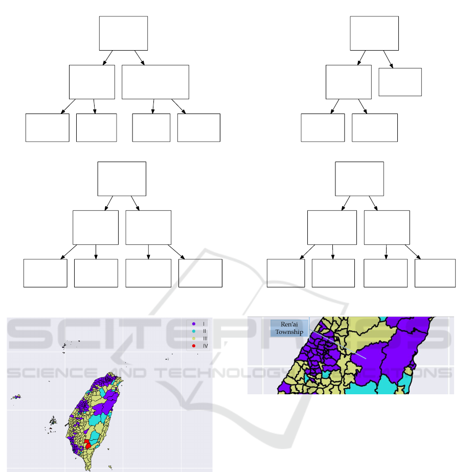
After assigning classes to all samples, we built one

decision tree. We randomly selected 90 percent of

samples (331 samples) as the training dataset to train

the decision tree model in each round. We set the max

depth of the decision trees to two to identify the two

most effective features. The four decision trees are

given in Figure 1.

From Figure 1, we can see that they all choose

the same feature in their root nodes. This feature is

the ratio of the elderly population in the area. The

next features in the decision tree in the four rounds are

respectively the ratio of infant and toddler population,

the ratio of the elder children (c

), and the ratio of the

young adult (a

) in the population.

We use the four decision trees to recognize all the

areas in Taiwan. Each decision uses the same set of

areas but with different age groups. As mentioned in

Section 4.3, this setting makes the younger and elder

age groups more important in our experiment. The

same area may be an urban or rural area by different

decision trees. An area may be classiﬁed as an urban

or rural area with one, two, three, or four times. We

use the four classiﬁcation results to classify the areas

into three classes, the urban area, the suburban area,

and the rural area, by voting. Speciﬁcally, if an area

is classiﬁed as urban by three or four decision trees,

this area is assigned to an urban area. Similarly, if an

area is classiﬁed to non-urban by three or four deci-

sion trees, this area is assigned to a rural area. Finally,

an area classiﬁed as urban and non-urban for both two

times is assigned to a suburban area, and we ignored

the uninhabited areas in the dataset.

The map of divisions of Taiwan colored according

to our results is given in Figure 2. Type I, II, and III

are the urban, the suburban, and the rural area decided

by the voting results, respectively. Type IV are those

areas we ignored. These four classes represent areas

DATA 2022 - 11th International Conference on Data Science, Technology and Applications

420

a_2 <= 0.139

entropy = 0.97

samples = 331

value = [199, 132]

class = y[0]

c_0 <= 0.099

entropy = 0.608

samples = 154

value = [23, 131]

class = y[1]

True

elementary_ratio <= 0.673

entropy = 0.05

samples = 177

value = [176, 1]

class = y[0]

False

entropy = 0.259

samples = 137

value = [6, 131]

class = y[1]

entropy = 0.0

samples = 17

value = [17, 0]

class = y[0]

entropy = 0.0

samples = 1

value = [0, 1]

class = y[1]

entropy = 0.0

samples = 176

value = [176, 0]

class = y[0]

a_2 <= 0.164

entropy = 0.988

samples = 331

value = [187, 144]

class = y[0]

c_1 <= 0.124

entropy = 0.835

samples = 196

value = [52, 144]

class = y[1]

True

entropy = 0.0

samples = 135

value = [135, 0]

class = y[0]

False

entropy = 0.169

samples = 40

value = [39, 1]

class = y[0]

entropy = 0.414

samples = 156

value = [13, 143]

class = y[1]

a_2 <= 0.136

entropy = 0.992

samples = 331

value = [183, 148]

class = y[0]

a_0 <= 0.115

entropy = 0.594

samples = 146

value = [21, 125]

class = y[1]

True

a_0 <= 0.155

entropy = 0.542

samples = 185

value = [162, 23]

class = y[0]

False

entropy = 0.998

samples = 36

value = [19, 17]

class = y[0]

entropy = 0.131

samples = 110

value = [2, 108]

class = y[1]

entropy = 0.344

samples = 171

value = [160, 11]

class = y[0]

entropy = 0.592

samples = 14

value = [2, 12]

class = y[1]

a_2 <= 0.133

entropy = 0.989

samples = 331

value = [186, 145]

class = y[0]

weekday <= 945.0

entropy = 0.474

samples = 138

value = [14, 124]

class = y[1]

True

a_0 <= 0.132

entropy = 0.496

samples = 193

value = [172, 21]

class = y[0]

False

entropy = 0.0

samples = 6

value = [6, 0]

class = y[0]

entropy = 0.33

samples = 132

value = [8, 124]

class = y[1]

entropy = 0.159

samples = 173

value = [169, 4]

class = y[0]

entropy = 0.61

samples = 20

value = [3, 17]

class = y[1]

Figure 1: Decision trees of all four clustering results.

Figure 2: Final results of administrative regions in Taiwan.

that have similar epidemic transmission conditions.

6 DISCUSSION

We examined the results given in Figure 2. We found

that some areas are considered non-urban areas or

suburban areas in Taiwan but are classiﬁed as subur-

ban areas or urban areas in our result. Two such ex-

amples, Ren’ai Township in Nantou and Xiulin Town-

ship in Hualien, are given in Figure 3. These two ar-

eas are usually considered non-urban areas. We found

that both townships are on the route of the Central

Figure 3: The regions affected by the Central Cross-Island

Highway.

Cross-Island Highway, one of the highways connect-

ing the west and the east areas of Taiwan. Road in-

frastructure may be why the condition of epidemic

transmission in the two townships is similar to that

in urban areas.

Figures 4 and 5 give some townships with similar

situation to what we mentioned above. In Figure 4,

Daxi District and Datong Township are not urban ar-

eas in Taiwan, but our model recognized them as ur-

ban areas. Similarly, Haiduan Township in Figure 5 is

a rural area in Taiwan, and this township is recognized

as a suburban area in our result. Provincial Highway 7

of Taiwan passes Daxi District and Datong Township,

and Provincial Highway 20 of Taiwan passes Haiduan

Township. Road infrastructure may play an important

role in epidemic transmission.

Using Machine Learning Methods and the Inﬂuenza Simulation System to Explore the Similarities of Taiwan’s Administrative Regions

421

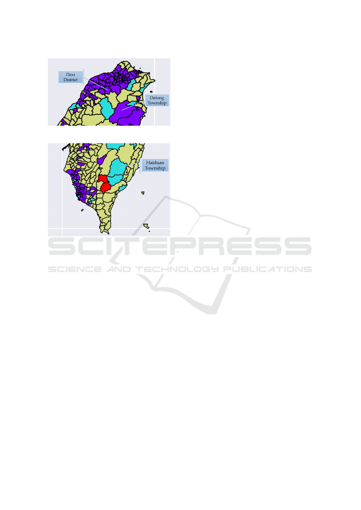
Figure 4: The regions affected by the North Link Highway.

Figure 5: The regions affected by the South Link Highway.

7 CONCLUSION

We used clustering methods to cluster the samples

generated by the simulation system of infectious dis-

eases to cluster administrative regions with similar

conditions of epidemic transmission. We also iden-

tiﬁed urban and non-urban areas by clustering meth-

ods. The result of clustering was then used to label

the samples to build decision trees. From the deci-

sion trees we built, we found age distributions are the

important features distinguishing the rural and urban

areas. In addition, by further analyzing the result, we

also found that road infrastructure may be important

to epidemic transmission.

ACKNOWLEDGMENT

This study was supported in part by MOST, Taiwan

by Grants 108-2221-E-001-011-MY3 and 110-2222-

E-033-005-.

REFERENCES

Balcan, D., Colizza, V., Gonc¸alves, B., Hu, H., Ramasco,

J. J., and Vespignani, A. (2009). Multiscale mobility

networks and the spatial spreading of infectious dis-

eases. Proceedings of the National Academy of Sci-

ences, 106(51):21484–21489.

Bargain, O. and Aminjonov, U. (2020). Trust and com-

pliance to public health policies in times of covid-19.

Journal of Public Economics, 192:104316.

Bijkerk, P., van Lier, E., van Vliet, J., and Kretzschmar,

M. Effecten van vergrijzing op infectieziekten. Ned

Tijdschr Geneeskd 2010;154:A1613.

Breiman, L., Friedman, J. H., Olshen, R. A., and Stone,

C. J. (1984). Classiﬁcation and Regression Trees.

Wadsworth and Brooks, Monterey, CA.

Chang, H., Chuang, J., Chern, T., Stein, M., Coker, R.,

Wang, D., and Hsu, T. (2014). A comparison be-

tween a deterministic, compartmental model and an

individual based-stochastic model for simulating the

transmission dynamics of pandemic inﬂuenza. In 4th

International Conference On Simulation And Model-

ing Methodologies, Technologies And Applications,

SIMULTECH 2014, Vienna, Austria, August 28-30,

2014, pages 586–594. IEEE.

Heald-Sargent, T., Muller, W. J., Zheng, X., Rippe, J., Patel,

A. B., and Kociolek, L. K. (2020). Age-Related Dif-

ferences in Nasopharyngeal Severe Acute Respiratory

Syndrome Coronavirus 2 (SARS-CoV-2) Levels in

Patients With Mild to Moderate Coronavirus Disease

2019 (COVID-19). JAMA Pediatrics, 174(9):902–

903.

Lenzen, M., Li, M., Malik, A., Pomponi, F., Sun, Y.-

Y., Wiedmann, T., Faturay, F., Fry, J., Gallego, B.,

Geschke, A., et al. (2020). Global socio-economic

losses and environmental gains from the coronavirus

pandemic. PloS one, 15(7):e0235654.

Opendata platform (2022). Opendata platform. https://data.

gov.tw/en. Online; access 22 March, 2022.

Prothero, R. M. (1977). Disease and mobility: a neglected

factor in epidemiology. International journal of epi-

demiology, 6(3):259–267.

Quinlan, J. R. (1986). Induction of decision trees. Machine

Learning, 1:81–106.

Quinlan, J. R. (1993). C4.5: Programs for Machine Learn-

ing. Morgan Kaufmann Publishers Inc., San Fran-

cisco, CA, USA.

Ward, J. H. (1963). Hierarchical grouping to optimize an

objective function. Journal of the American Statistical

Association, 58(301):236–244.

World Health Organization (2010). Inﬂuenza a (h1n1)

pandemic 2009 - 2010. https://www.who.int/

emergencies/situations/inﬂuenza-a-(h1n1)-outbreak.

Online; access 22 March, 2022.

World Health Organization (2022). Coronavirus dis-

ease (covid-19) pandemic. https://www.who.int/

emergencies/diseases/novel-coronavirus-2019. On-

line; access 22 March, 2022.

DATA 2022 - 11th International Conference on Data Science, Technology and Applications

422