Learning Optimal Robot Ball Catching Trajectories Directly from the

Model-based Trajectory Loss

Arne Hasselbring

, Udo Frese

1,2

and Thomas R

ofer

1,2

Deutsches Forschungszentrum f

ur K

unstliche Intelligenz, Cyber-Physical Systems, Bremen, Germany

Universit

at Bremen, Fachbereich 3 – Mathematik und Informatik, Bremen, Germany

Keywords:

Trajectory Optimization, Machine Learning, Robot Dynamics.

Abstract:

This paper is concerned with learning to compute optimal robot trajectories for a given parametrized task. We

propose to train a neural network directly with the model-based loss function that deﬁnes the optimization

goal for the trajectories. This is opposed to computing optimal trajectories and learning from that data and

opposed to using reinforcement learning. As the resulting optimization problem is very ill-conditioned, we

propose a preconditioner based on the inverse Hessian of the part of the loss related to the robot dynamics.

We also propose how to integrate this into a commonly used dataﬂow-based auto-differentiation framework

(TensorFlow). Thus it keeps the framework’s generality regarding the deﬁnition of losses, layers, and dataﬂow.

We show a simulation case study of a robot arm catching a ﬂying ball and keeping it in the torus shaped bat.

The method can also optimize “voluntary task parameters”, here the starting conﬁguration of the robot.

1 INTRODUCTION

Motion planning (LaValle, 2006) is one of the most

central issues for moving autonomous systems, let it

be robot manipulators (Singh and Leu, 1991), autono-

mous vehicles (Lim et al., 2018) or spacecraft (Niko-

layzik et al., 2011). In some scenarios, obstacle ge-

ometry is the most difﬁcult part, e.g. when a robot

mounts a bulky part in a motor compartment. Some-

times it is closed-loop reactivity, e.g. when balancing.

And sometimes the dynamics of the system pose the

largest challenge, e.g. when the system is operated

close to its technical and physical limits and motion

planning shall get the best performance out of these

limits. Our long term goal is to perform ball sports

tasks with a two-arm robot (Fig. 1), such as catching,

throwing, or juggling. These require very dynamic

movements, as “gravity is not waiting for you”, and

bring typical industrial robots to their limit.

1.1 An Optimization View

Often such a planning task is formulated as an opti-

mization problem:

∗

(a) = argmin

1...T

∈R

T ×D

L (a,q) (1)

Here q

1...T

is the trajectory, deﬁning a D-dimensional

(joint) position vector per discretized timestep and

f(q)

(q)

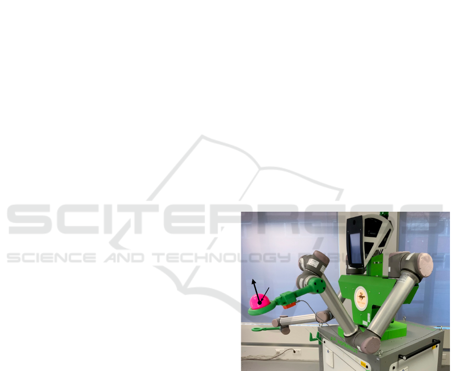
Figure 1: Our long term goal is to perform ball sports tasks,

like throwing, catching, juggling, with this two-arm robot.

The abstract and passive design of the torus-shaped bat im-

poses constraints to avoid losing the ball.

L (a,q) is the loss function that deﬁnes the optimiza-

tion goal. The loss function includes a model of the

system (here robot dynamics) and a formalization of

the task to be achieved, e.g. catching a ball. It also

includes constraints, e.g. position, velocity, accelera-

tion, or torque limits, abstractly by setting L (a,q) =

∞ for infeasible q, or concretely by including a barrier

function. The loss depends on some task parameters a

describing the concrete task instance, e.g. a goal pose

or – in our case – the trajectory of an incoming ball.

Hasselbring, A., Frese, U. and Röfer, T.

Learning Optimal Robot Ball Catching Trajectories Directly from the Model-based Trajectory Loss.

DOI: 10.5220/0011279000003271

In Proceedings of the 19th International Conference on Informatics in Control, Automation and Robotics (ICINCO 2022), pages 201-208

ISBN: 978-989-758-585-2; ISSN: 2184-2809

201

If the task input a is not available beforehand, this

optimization creates a delay before the motion can

start and is computationally challenging despite mod-

ern algorithms and libraries, e.g. CasADI (Andersson

et al., 2019) and WORHP (Nikolayzik et al., 2011).

Because of this and the recent success of machine

learning, it is promising to learn a mapping from

a 7→ q

∗

, e.g. with a neural network. One could use

supervised learning with computed (a,q

∗

(a)) pairs:

∗

= argmin



(a) − q

∗

(a)



(2)

Here θ are the learned parameters of a neural net-

work q

(a) that maps a 7→ q

∗

. The E

is an expected

value with respect to a distribution (practically a set)

of training data for a. Alternatively, one could also

run reinforcement learning with L (a,q) as reward.

1.2 Learning Directly from the

Trajectory’s Loss

However, in this paper we investigate to use the model

based L (a,q) directly as loss for the learning process:

∗

= argmin

[L (a,q

(a))] (3)

The system and task model are part of L and thus part

of the learning optimization. Typically, such losses

are differentiable as needed for gradient descent. This

approach appears promising, because:

First, unlike (2), (3) considers which direction

of deviation from the optimum affects the loss how

much. So it aims for the best solution, not the one

closest to the optimum. This is very relevant for loss

terms depending on derivatives of q (Sec. 4.1).

Second, in reinforcement learning every roll-out

produces – roughly speaking – a single total loss

value. The distribution of the loss over timesteps is

not that helpful, because of the delayed reward prob-

lem. In contrast, gradient descent on (3) produces one

derivative with respect to every entry of q. Thus the

approach takes more information from the loss, utiliz-

ing that a model-based loss can be differentiated.

Third, sometimes the task input has a voluntary

part a

that can be chosen by the system but only

before the remaining a

¯v

arrives (a = (a

¯v

)). For

instance, we can choose the starting conﬁguration

= q

, but only before the ball approaches, i.e. in-

dependent of a

¯v

, best on average. These parameters

can be optimized along in (3) as arg min

θ,a

.. ., which

is not possible in (1), that considers only a single task

instance.

However, (3) is more difﬁcult to optimize than (2),

because it is conditioned worse (Sec. 4.1). Therefore,

we propose an inverse Hessian preconditioning of the

robot dynamics to make it tractable for common gra-

dient optimizers. Overall, this paper contributes:

• A method to learn trajectory optimization prob-

lems directly from the trajectory’s loss and opti-

mizing voluntary task inputs along for loss func-

tions involving robot dynamics.

• The concept and implementation, how this

method can be integrated into a common dataﬂow

auto-differentiation framework (TensorFlow).

• A simulation case study, for the task of catching

ﬂying balls, including full robot dynamics, choice

of starting conﬁguration, and the mechanical con-

straints for the ball to stay in the bat (Fig. 1).

The paper is structured as follows: After related work

we introduce the generic parts of a robot trajectory

loss refering to joint velocities and torques (Sec. 3),

and propose the inverse Hessian preconditioner and

its integration into TensorFlow (Sec. 4). Then, we

study the case of ball catching (Sec. 5), and conclude.

2 RELATED WORK

Rao (2014) gives a survey on trajectory optimization.

He distinguishes between indirect methods, where the

control action is the variable to be optimized, and di-

rect methods, where the trajectory itself is optimized.

This part is relevant here, as we substitute the non-

linear trajectory optimizer by a neural network. As

Rao says, “Typically, optimal trajectory generation

is performed off-line, that is, such problems are not

solved in real time nor in a closed-loop manner.”,

showing the need for efﬁcient approximations.

Toussaint (2017) gives an excellent tutorial on

the Newton method applied to trajectory optimiza-

tion. He highlights relations to other ﬁelds, which all

use minimization of quadratic functions as a common

core, namely Simultaneous Localization and Map-

ping (SLAM), optimal control and probabilistic infer-

ence. In particular, he points out the bandmatrix struc-

ture of the Hessian, which we utilize in Section 4.1.

Kurtz et al. (2022) developed a controller that

makes a falling Mini Cheetah robot always land on

its feet, as cats do. They use an ofﬂine trajectory op-

timizer to either map the current state to joint torques

or to map the initial state to a whole trajectory (the

so-called reﬂex) and trained two neural networks on

that. Experiments showed that the second network

performed much better. This resembles the approach

presented in this paper, but optimizing (2), not (3).

Mansard et al. (2018) conﬁrm these ﬁndings.

They use a neural network inside a probabilistic

ICINCO 2022 - 19th International Conference on Informatics in Control, Automation and Robotics

202

roadmap framework to learn a mapping from task in-

put (start state, goal state, environment) to a) a control

action and b) a trajectory. They use supervised learn-

ing with ground truth from a model-based optimizer

and report that b) works better. Overall they aim at a

good initial guess to speed up convergence.

Sch

uthe and Frese (2015) use full dynamic Model

Predictive Control in real-time at 50 Hz to bat a ball.

However, their robot only has three joints.

auml et al. (2010) optimize a ball catching tra-

jectory for a 7-DOF arm utilizing the redundancy both

of the robot itself and the task in 10 ms on average

(2.2 GHz quad-core Xeon). The optimization is kine-

matic, with joint acceleration instead of torque limits.

Hence, they actually optimize the catching conﬁgura-

tion using the optimal trapezoidal trajectory.

A large body of work considers kinematic motion

planning, without taking dynamics into account but in

geometrically complex environments. An example of

this class is Schulman et al. (2013) and Ratliff et al.

(2009), who showed how to integrate geometric ob-

stacles into an optimization-based approach.

3 DYNAMIC ROBOT LOSS

Every trajectory that is executed on a robot should

comply with the robot’s physical limits and also min-

imize the required control effort. This is encoded in

the dynamic robot loss deﬁned in terms of torques

and joint velocities. Besides the optimization variable

1...T

, this depends on boundary conditions as well.

The trajectory is extended by q

−1...0

at the start, which

represent the current state of the robot (in this pa-

per initial conﬁguration, no velocity). The robot shall

stop ﬁnally, so q

is repeated in the end q

T +1

= q

forcing the last velocity to zero. Given the now ex-

tended discrete trajectory q

−1...T +1

, the continuous

q(t) is deﬁned by linear interpolation:

q(t) = frac(t)q

⌊t⌋+1

+ (1 − frac(t))q

⌊t⌋

(4)

q(t) is then the difference quotient of the adjacent q

q(t) =

⌊t⌋+1

− q

⌊t⌋

∆T

(5)

and similarly, the accelerations (which are only

needed at integer timesteps) are

q(t) =

t+1

+ q

t−1

− 2q

∆T

. (6)

τ : R

× R

→ R

is the vector of torques per

joint that can be obtained via inverse dynamics from

the joint angles, velocities, and accelerations. In the

following, τ

∗

∈ R

and

∗

∈ R

are the speciﬁed

maximum joint torques and velocities, respectively.

The main loss component that smoothens the en-

tire trajectory is the sum of squared torques, normal-

ized by their maximum values:

(q) =

∑

t=0

∑

j=1

(q(t),

q(t),

q(t))

∗

(7)

The other two components address the hard limits on

torques and velocity. Deﬁne the function

clip(x,c) =

max(x − c, 0)

1 − c

(8)

that maps values below c to 0 and scales them to map

1 to 1. Then, the following loss component penalizes

violations of the maximum torques and velocities:

∗

(q) =

∑

t=0

∑

j=1

clip

|τ

(q(t),

q(t),

q(t))|

∗

(9)

˙q

∗

(q) =

∑

t=0

∑

j=1

clip

| ˙q

(t)|

˙q

∗

˙q

∗

(10)

The thresholds c

∗

˙q

∗

< 1 deﬁne a fraction of the

actual limits at which the penalty starts, as the terms

only deﬁne a soft, not a hard limit (cf. Sec. 5.2).

The complete dynamic loss is constructed as a

weighted sum of its components:

dyn

(q) = α

(q) + α

∗

(q) + α

˙q

∗

˙q

∗

(q) (11)

4 INVERSE HESSIAN

PRECONDITIONING

4.1 The Conditioning Problem

The dynamic loss L

dyn

has directions of very large

curvature due to the terms related to

q (and τ), while

typical task losses related to q create directions of

much smaller curvature. To see this, consider as illus-

tration the following simpliﬁed loss for just one joint:



◦





100

◦



∑

t=2



¨q(t)

100

◦



(12)

It demands q

, q

100

and ¨q to be zero and punishes 1

◦

as much as 100

◦

−2

. The optimum is clearly q

= 0.

If we change all q

together by δq/10 (a change

of norm δq), the loss grows by 2/100 δq

. If we

change one q

in the middle by δq, the loss grows by

+(−2)

(100

◦

∆T

)

δq

≈ 1.5 · 10

δq

, with ∆T = 125 s

−1

This is called bad conditioning and the ratio between

the smallest and the largest curvature is the condition

Learning Optimal Robot Ball Catching Trajectories Directly from the Model-based Trajectory Loss

203

number ≈ 7 · 10

. For our actual dynamic loss (L

dyn

(11) with weights given in Section 5.4) the condition

number is even ≈ 2 · 10

This impedes ﬁrst-order methods, e.g. gradient de-

scent, because the step rate is limited by the direction

of highest curvature, making steps in the direction of

lowest curvature extremely small.

While ﬁrst-order methods are typical for deep

learning (and hence well supported in prominent soft-

ware frameworks), trajectory optimization therefore

commonly uses second-order methods (Toussaint,

2017). Properly using Newton’s method requires the

full Hessian of the loss function w.r.t. the parameters.

This can, in general, be intractable. Therefore, many

quasi-Newton methods exist, such as L-BFGS (Liu

and Nocedal, 1989), which estimate an approximate

inverse Hessian from a sequence of gradients. Modi-

ﬁcations (Schraudolph et al., 2007) are also applicable

to stochastic problems.

4.2 Preconditioning

However, we can take a different approach: Recall

that L

dyn

is a sum of squares, so it can be written as

dyn

(q) =

∥r(q)∥

(13)

with r(q) ∈ R

3(T +1)D

being a “residual” vector, each

element corresponding to one of the summands in

Equations 7–10. This residual function has a Jaco-

bian J

(q), which has to be calculated anyway for the

gradient and we can construct the pseudo-Hessian

H = J

(q)

⊤

(q) (14)

of L

dyn

w.r.t. the trajectory q in the common Gauß-

Newton approach. The idea is then to use this matrix

as a preconditioner for the gradient of the loss w.r.t.

q and propagate the preconditioned gradient further

back through the neural network as in ﬁrst-order gra-

dient descent. Fortunately, H is symmetric banddiag-

onal with a 3D − 1 wide band, because each timestep

only relates to its two neighbors (Toussaint, 2017,

§2.3). This allows to solve for this matrix with a com-

putation time linear in T .

The idea to only compute the pseudo-Hessian of

the dynamics loss and not of the total loss corresponds

to CHOMP’s (Ratliff et al., 2009) idea to only include

a smoothing loss in the pseudo-Hessian, however we

refer to the torques instead of joint accelerations, i.e.

consider the robot dynamics. As they say: “[..] It is

useful to interpret the action of the inverse operator

−1

] as spreading the gradient across the entire tra-

jectory so that updating by the gradient decreases the

cost [..] while retaining trajectory smoothness.”

projectile

motion

catch

)

task

loss

dyn.

loss

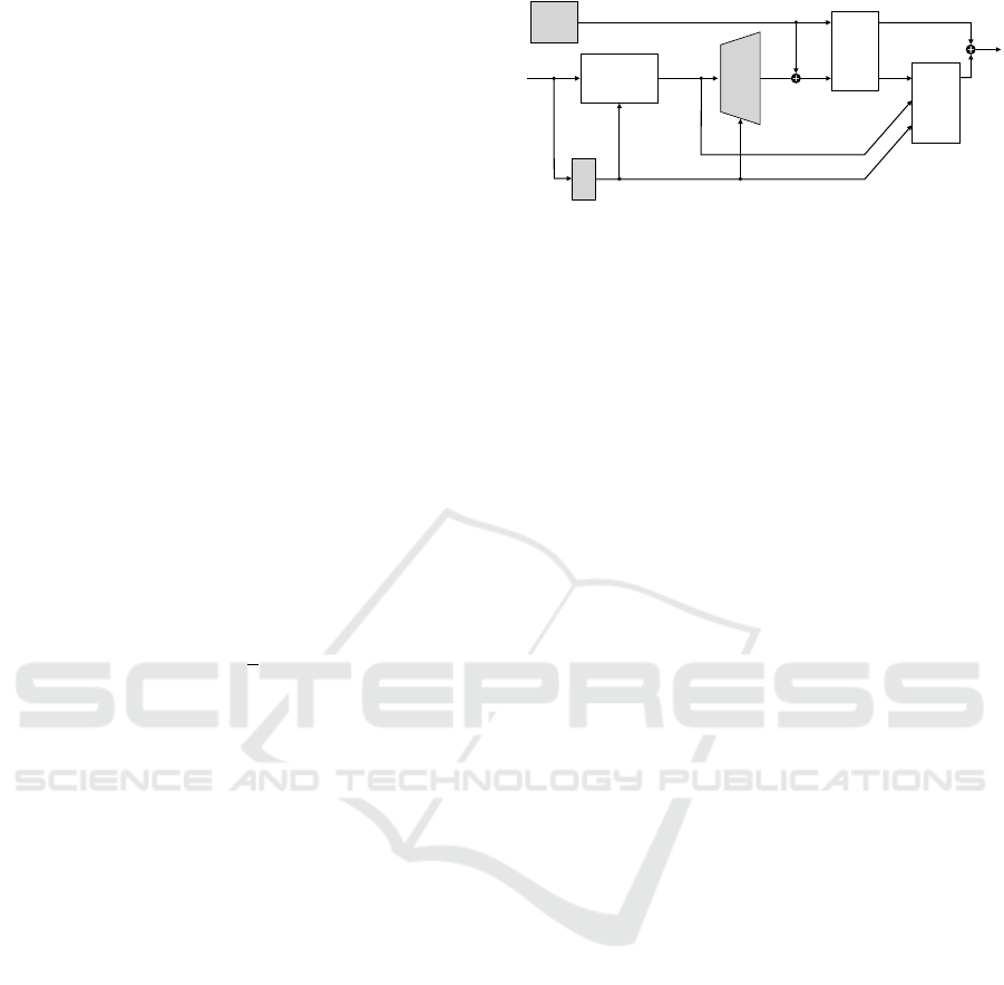
Figure 2: Dataﬂow of the system during training. The

shaded boxes contain learnable parameters while clear

boxes are model-based. During execution, the loss boxes

are removed.

Note that while only the dynamic part of the loss

function L

dyn

is used to construct the Hessian, the

whole loss function (L

dyn

+ L

task

) needs to be mul-

tiplied with the inverse Hessian, because

0 = ∇(L

dyn

+ L

task

) ⇔ 0 = H

−1

∇(L

dyn

+ L

task

)

⇎ 0 = H

−1

∇L

dyn

+ L

task

, (15)

i.e. optima can change otherwise.

4.3 Integration into TensorFlow

There is a software engineering challenge in inte-

grating the presented preconditioning into a dataﬂow

driven auto-differentiation framework, such as Ten-

sorFlow (Abadi et al., 2015). We want to develop the

neural network part q

(a), deﬁne task loss functions

with speciﬁc formulas, and use predeﬁned optimizers

as usual. Still, we want to use the established C++

library Pinocchio (Carpentier et al., 2021) to compute

τ (inverse robot dynamics) and ∇τ and use special-

ized C++ code to efﬁciently build and decompose the

band matrix H for the preconditioner. The solution is

a “robot dynamics” block (Fig. 2) that takes the tra-

jectory q including initial conditions q

−1

, along

with some attributes such as the path to the URDF

robot model. In the forward pass, the block just cal-

culates the dynamic losses L

∗

, and L

˙q

∗

. However,

it additionally outputs a copy of the input q, which

further loss calculations must use, such as L

task

. Be-

cause of this output, the block receives ∇L

task

during

the gradient computation in the backward pass and

can apply H

−1

to it. The user must take care that

the loss outputs of this function appear only linearly

in the total loss function, as otherwise the pseudo-

Hessian will be wrong. The block is technically a

Python wrapper function with custom gradients for

two TensorFlow C++ ops, one each for the forward

and backward pass. The implementation is available

at https://github.com/DFKI-CPS/tf-dynamics-op.

ICINCO 2022 - 19th International Conference on Informatics in Control, Automation and Robotics

204

5 BALL CATCHING CASE STUDY

As a case study for our trajectory optimization ap-

proach, we consider a ball catching robot. This is a

challenging task because several constraints have to

be met: The ball must be hit at the right time, with the

right velocity and rotation, and be kept from leaving

the bat again. This is on top of the general dynamic

feasibility and “elegance” of the trajectory.

Our scenario is episodic, i.e. the robot starts from

a stationary initial joint conﬁguration q

, which is the

same for all attempts, and included in the optimiza-

tion. As input, the system gets the initial ball posi-

tion p ∈ R

and velocity

p ∈ R

, e.g. from a tracking

system not considered here. The output of the sys-

tem is a trajectory, i.e. a sequence of T sets of joint

angles q

1...T

∈ R

T ×D

that catches the ball and subse-

quently balances the ball until stopping. The system

can choose when to catch the ball, and therefore the

state along the ball trajectory. For instance, a later

time will make the ball be closer and lower and its

velocity faster and steeper (Fig. 2).

5.1 Robot Model

Although this work is carried out entirely in simu-

lation, we still model the setup after the real robot

in Figure 1. It is a pi4 workerbot with two 6-DOF

Universal Robots UR10 CB2 collaborative robot arms

mounted on its “shoulders”. They can be controlled at

125Hz (∆T = 0.008 s), with joint velocity commands.

The robot has three types of motors: The ﬁrst type

is used for the two shoulder joints (v

∗

1,2

= 120

◦

−1

∗

1,2

= 330 Nm), the second for the elbow joint (v

∗

180

◦

−1

, τ

∗

= 150 N m), and the third for the three

wrist joints (v

∗

4,5,6

= 180

◦

−1

, τ

∗

4,5,6

= 56 Nm). A

model of the mass distribution is available, but to

match the torques the UR10 itself calculates, addi-

tional torques proportional to the accelerations have

to be added, probably to account for motor inertia. We

determined those factors experimentally to be 7kg m

for the shoulder joints, 2 kgm

for the elbow joint,

and 0.62 kgm

for the wrist joints. Considering the

torques instead of plain joint accelerations is neces-

sary, because the upper arm joints need to lift a sig-

niﬁcantly higher weight. Keeping the torque limits

is particularly important, because the real UR10, in-

stead of just limiting the current, will enter an error

state upon violating these.

The “hands” of the robot are torus-shaped with

major

= 47mm and r

minor

= 12.5mm.

Given a joint conﬁguration q ∈ R

, f, R

and J

represent the forward kinematics of the manipulator

in the global frame, speciﬁcally f : R

→ R

is the

ball’s center on the bat, R

: R

→ R

is the direction

vector orthogonal to the torus’ plane, and J : R

→

3×D

is the Jacobian of f (Fig. 1).

5.2 Task Loss

The task loss’ inputs are the trajectory q

1...T

, the de-

sired catch time point t

catch

, and the ball’s predicted

state at the catch time (p

catch

) ∈ R

×R

. It has

the following sum-of-squares-type components:

Position: The ball must be on the bat at the desired

catch time.

(q) = ∥f(q(t

catch

)) − p

catch

∥

(16)

Velocity: The velocity of the ball must match the

velocity of the bat at the catch time, up to a given fac-

tor c

< 1 (we assume that some kinetic energy can be

absorbed on impact, making it an inelastic collision).

˙p

(q) = ∥J(q(t

catch

))

q(t

catch

) − c

catch

∥

(17)

Rotation: The bat’s z axis must be aligned with the

ball velocity’s direction at the catch time (rotation

around the axis through the bat is arbitrary), such that

ideally, the ball touches the bat evenly.

(q) = ∥R

(q(t

catch

)) × −

catch

∥

(18)

Note this theoretically allows two optimal solutions

pointing in opposite directions, i.e. while R

and

catch

should be pointing in opposite directions, they

could as well point to the same. This is prevented by

other loss components and initial conditions.

Balance: Once the ball has collided with the bat, the

ball must be kept in position by a reaction force from

the bat, which can only act from within the torus. Oth-

erwise it would fall out. This imposes an upper bound

ball

max

minor

major

Figure 3: Cross-section of the tilted bat with a ball. The

reaction force acting on the ball’s center (here only counter-

ing gravity) must stay within the θ

max

cone around R

Learning Optimal Robot Ball Catching Trajectories Directly from the Model-based Trajectory Loss

205

max

on the angle between the direction R

(q(t)) and

the reaction force F

(t), where

cos(θ

max

) =

minor

+ r

ball

)

− r

major

minor

+ r

ball

(19)

and (with g being the gravity vector):

(t)

p(t) − g (20)

p(t) is calculated as second-order difference quotient

in Cartesian space (to avoid needing the Hessian of

the forward kinematics) and implicitly captures q(t),

although we actually do not backpropagate the gradi-

ent through this:

p(t) =

f(q(t + 1)) + f(q(t − 1)) − 2f(q(t))

∆T

(21)

As hard constraint, the balance condition is (Fig. 3)

cos(θ) =

(t)

⊤

(q(t))

∥F

(t)∥

≥ cos(θ

max

). (22)

Again, q is implicitly captured in θ, although here it

does receive a gradient. For differentiability, the loss

is a penalty, i.e. it is 0 below a speciﬁed fraction (c

)

of the limit angle θ

max

(q) =

∑

t=⌈t

catch

⌉

max



∥F

(t)∥

(cos(θ

max

) − c

cos(θ)),0



(23)

The complete task-speciﬁc loss function is:

task

= α

+ α

˙p

+ α

(24)

5.3 Network Architecture

There are two neural networks in the system (Fig. 2):

One produces the desired catch time point t

catch

from

the initial ball state, while the other produces the tra-

jectory from the catch time point and the predicted

ball state at that time.

By choosing a catch time, the network can utilize

an additional degree of freedom, namely a shift along

the trajectory to ﬁnd the point where it is most con-

venient to catch the ball. It has to output this time

explicitly and the loss assesses whether the ball and

trajectory at t

catch

are suitable for that.

The prediction of the catch time is subdivided into

an analytic component that calculates a base time, and

a neural network adding an offset. The base time is

To prevent self-collisions, we added another quadratic

term limiting the shoulder lift angle.

Table 1: Layers of the trajectory network. Residual lay-

ers add their input to their output. The last column states

whether the catch time is concatenated to the layer’s input.

Layer Units Activation Residual Time

1 20 leaky ReLU no no

2 100 leaky ReLU no yes

3 101 leaky ReLU yes yes

4 102 leaky ReLU yes yes

5 150 leaky ReLU no yes

6 D · T linear no no

chosen as the time when the ball crosses the z = 0

plane (a bit below shoulder level).

base

= −

˙p

0,z

˙p

0,z

− 2p

0,z

(25)

The initial ball state is then propagated to this time

and fed into a neural network together with t

base

. All

values are shifted to lie around 0. The catch time net-

work has three dense layers with 10, 5, and 1 units, re-

spectively. The ﬁrst two layers are activated by leaky

ReLU, while the last one uses tanh. This offset is then

scaled to a certain range (we used the factor 0.15) and

added to t

base

to obtain t

catch

After t

catch

has been determined, the actual ball

state at catch time (p

catch

) is calculated, which

is used as input for the trajectory network and refer-

ence for the task loss.

The architecture of the trajectory network is de-

scribed in Table 1. The input layer gets only the ball

state, and t

catch

is injected in later layers. The out-

put of the last layer is added to the broadcasted start

angles to form the trajectory that enters the loss func-

tion. This way, both the start angles and the trajectory

network receive gradients. The length of the trajec-

tory is ﬁxed to T = 225 timesteps (1.8 s).

5.4 Training Process

From the external perspective (ignoring the precon-

ditioner hidden in the dynamics block), the entire

computation graph (i.e. including both neural net-

works and the start conﬁguration) is trained with

plain stochastic gradient descent for 8000 epochs

over batches of 16 elements. The inputs (p

)

are generated as follows: First a target position is

sampled from a subregion of the reachable space

of the bat [0.8,1.2] × [0,0.6] × [−0.1,0.2][m]. In-

dependently, a target velocity is uniformly sam-

pled from the range [−3.7, −2.7] × [−0.5, 0.5] ×

[−4.1,−3.9][ms

−1

]. These are traced back by a ﬁxed

time (1s) according to projectile motion. Note that

this does not exactly cancel out with the projectile

ICINCO 2022 - 19th International Conference on Informatics in Control, Automation and Robotics

206

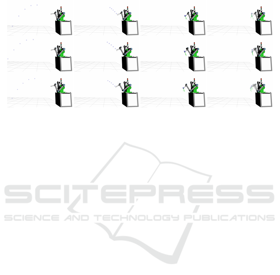
Figure 4: Kinematic visualization of three generated trajectories (from left to right) with different initial ball states. Contact

dynamics are not simulated here, instead the ball is attached to the bat at the catch time. The balance constraint is visualized

by the direction of the force (−F

) with a green arrow in the right two frames. A video of multiple trajectories can be found

at https://tinyurl.com/e4dk7m6d.

motion block in the system, since the system can ad-

just the time point and actual catch position.

The learning rate starts at 5 · 10

−4

and decays ev-

ery 100 epochs by a factor of 0.9. The training suc-

cess is highly sensitive to these learning rate(s).

The weights of the velocity loss α

˙p

and balance

loss α

are gradually blended in during training. They

start at 0 and increase by 0.01 in every epoch in which

is below 0.002, up to a maximum value of 10. The

idea is that in the ﬁrst epochs, the optimizer should

mainly try to get the trajectory to a rougly right po-

sition and rotation (i.e. solve inverse kinematics ﬁrst)

before turning to velocity and balance, which could

otherwise prevent the optimizer from getting there.

Similarly, the learning rate for the catch time network

is increased, so it starts learning only after the opti-

mizer has roughly reached the right position.

The other loss weights are ﬁxed at α

= 1, α

∗

= 1,

∗

= 5, α

= 1000, α

= 33. c

∗

, c

˙q

∗

and c

are set to

0.9 (penalties starting at 90% of the respective limits).

These values have been determined by trial and error.

5.5 Results

First of all, qualitative results in form of visualized

example trajectories and a video link are given in Fig-

ure 4. The trajectories are generally smooth and the

bat manages to arrive at the ball in time with suitable

rotation and velocity. However, as this is just a vi-

sualization without contact dynamics, we can’t draw

conclusions about the real ball-bat interaction.

Quantitatively, we can examine some metrics on

a “test set”, i.e. a grid over the input space consisting

of 50000 states. The mean loss (with α

˙p

= α

= 10)

over this set is 10.92. No trajectory violates the maxi-

mum torque/velocity constraints. However, the mean

error in catch position is quite high with 17.3 mm. We

assume that position errors larger than 10 mm would

cause the ball to bump out of the bat.

To improve the precision, we can calculate the a-

posteriori error p

catch

− f(q(t

catch

)) and run the tra-

jectory network again with a modiﬁed target position

catch

− f(q(t

catch

)). This assumes that the network

behaves locally consistent. Indeed, this reduces the

mean position error to 10.5mm.

In order to assess the inﬂuence of letting the op-

timizer choose the catch time, we train the system

(i.e. trajectory network and start conﬁguration) with-

out the catch time offset, i.e. setting t

catch

= t

base

. This

results in a mean loss of 11.17. Similarly, we can dis-

able optimization of the start conﬁguration and leave

it at a reasonable default guess. The resulting mean

loss over the test set is 10.96, which seems insigniﬁ-

cant compared to the value of 10.92 for the full prob-

lem. However, now some of the trajectories violate

the velocity limits. This indicates that the optimizer

actually utilizes the additional degrees of freedom.

The inference time using TensorFlow on a note-

book CPU is about 2ms including the reﬁnement step.

6 CONCLUSIONS & OUTLOOK

We have shown that it is possible to learn a mapping

from task input to optimal trajectory directly from

the trajectory’s loss, when the inverse Hessian of the

robot dynamics loss is used as preconditioner. This

can be implemented as a block in TensorFlow with

a special bypass output that allows to apply the pre-

Learning Optimal Robot Ball Catching Trajectories Directly from the Model-based Trajectory Loss

207

conditioner also to the other parts of the loss deﬁned

outside that block. The simulated ball catching case

study showed that this approach works in practice and

can optimize voluntary task parameters along with

learning the network, in our case the starting conﬁgu-

ration of the robot arm.

Future work will be to improve spatial precision

by a more general iteration and also to include a mov-

ing horizon scheme, which can handle “inﬁnite” tasks

such as juggling and can adapt to sensor input, e.g. a

change in ball prediction.

ACKNOWLEDGEMENTS

This work is partially funded by the German BMBF

– Bundesministerium f

ur Bildung und Forschung

project Fast&Slow (FKZ 01IS19072).

REFERENCES

Abadi, M. et al. (2015). TensorFlow: Large-scale machine

learning on heterogeneous systems. Software avail-

able from tensorﬂow.org.

Andersson, J. A. E., Gillis, J., Horn, G., Rawlings, J. B.,

and Diehl, M. (2019). CasADi: a software framework

for nonlinear optimization and optimal control. Math-

ematical Programming Computation, 11(1):1–36.

auml, B., Wimb

ock, T., and Hirzinger, G. (2010). Kine-

matically optimal catching a ﬂying ball with a hand-

arm-system. In 2010 IEEE/RSJ International Confer-

ence on Intelligent Robots and Systems, pages 2592–

2599. IEEE.

Carpentier, J., Valenza, F., Mansard, N., et al. (2015–

2021). Pinocchio: fast forward and inverse dy-

namics for poly-articulated systems. https://stack-of-

tasks.github.io/pinocchio.

Kurtz, V., Li, H., Wensing, P. M., and Lin, H. (2022).

Mini Cheetah, the falling cat: A case study in ma-

chine learning and trajectory optimization for robot

acrobatics. In 2022 IEEE International Conference

on Robotics and Automation (ICRA).

LaValle, S. M. (2006). Planning Algorithms. Cambridge

University Press.

Lim, W., Lee, S., Sunwoo, M., and Jo, K. (2018). Hierar-

chical trajectory planning of an autonomous car based

on the integration of a sampling and an optimization

method. IEEE Transactions on Intelligent Transporta-

tion Systems, 19(2):613–626.

Liu, D. C. and Nocedal, J. (1989). On the limited memory

BFGS method for large scale optimization. Mathe-

matical Programming, 45:503–528.

Mansard, N., del Prete, A., Geisert, M., Tonneau, S., and

Stasse, O. (2018). Using a memory of motion to efﬁ-

ciently warm-start a nonlinear predictive controller. In

2018 IEEE International Conference on Robotics and

Automation (ICRA).

Nikolayzik, T., B

uskens, C., and Wassel, D. (2011). Nonlin-

ear optimization in space applications with WORHP.

Technical Report Berichte aus der Technomathematik,

11-10, University of Bremen.

Rao, A. V. (2014). Trajectory optimization: A survey. In

Waschl, H., Kolmanovsky, I., Steinbuch, M., and del

Re, L., editors, Optimization and Optimal Control in

Automotive Systems, volume 455 of LNCIS, pages 3–

21. Springer.

Ratliff, N., Zucker, M., Bagnell, J. A., and Srinivasa, S.

(2009). CHOMP: Gradient optimization techniques

for efﬁcient motion planning. In 2009 IEEE In-

ternational Conference on Robotics and Automation

(ICRA).

Schraudolph, N. N., Yu, J., and G

unter, S. (2007). A

stochastic quasi-Newton method for online convex op-

timization. In 11th International Conference on Arti-

ﬁcial Intelligence and Statistics (AIstats), volume 2 of

PMLR, pages 436–443.

Schulman, J., Ho, J., Lee, A., Awwal, I., Bradlow, H., and

Abbeel, P. (2013). Finding locally optimal, collision-

free trajectories with sequential convex optimization.

In Robotics: Science and Systems, volume 9.

Sch

uthe, D. and Frese, U. (2015). Optimal control with

state and command limits for a simulated ball batting

task. In 2015 IEEE/RSJ International Conference on

Intelligent Robots and Systems (IROS), pages 3988–

3994. IEEE.

Singh, S. K. and Leu, M. C. (1991). Manipulator motion

planning in the presence of obstacles and dynamic

constraints. The International Journal of Robotics Re-

search, 10(2):171–187.

Toussaint, M. (2017). A tutorial on Newton methods for

constrained trajectory optimization and relations to

SLAM, Gaussian process smoothing, optimal con-

trol, and probabilistic inference. In Laumond, J.-P.,

Mansard, N., and Lasserre, J.-B., editors, Geometric

and Numerical Foundations of Movements, volume

117 of STAR, pages 361–392. Springer.

ICINCO 2022 - 19th International Conference on Informatics in Control, Automation and Robotics

208