Optimal Social Limitation Reduction under Vaccination and Booster

Doses

Paolo Di Giamberardino

and Daniela Iacoviello

Department of Computer, Control and Management Engineering, Sapienza University of Rome, Rome, Italy

Keywords:

Epidemic Modeling, COVID-19, Vaccination, Optimal Control, Social Behaviour.

Abstract:

In the paper an optimal control solution is provided for the containment of the number of infected individuals

in COVID-19 pandemic under vaccination campaign. The possibility to dynamically change the cost of the

controls according to the ongoing evolution within the design procedure allows to get great efforts in presence

of very serious disease conditions, saving resources otherwise. The different contribution of vaccinated and

unvaccinated individuals to the epidemic spread is investigated, optimising the controls which describe the

individual contact restrictions separately for the two classes and showing that it would have been possible

to reduce all the social limitations introduced by many governments for the vaccinated individuals since the

beginning of the vaccination campaign.

1 INTRODUCTION

COVID-19 is a sanitary emergency since January

2020 and the scientiﬁc community has started to

study the evolution and the spread of the infection

by means of mathematical models which had to fol-

low the changes and the novelties in the knowledge

of the illness, updated day by day, and in the pos-

sibility to ﬁght the virus, as for examples (Di Gi-

amberardino et al., 2021),(Giordano et al., 2020),

(Tang et al., 2020), (Di Giamberardino and Iacoviello,

2021), (Radulescu et al., 2020). In particular, since

the end of 2020, the availability of an effective vac-

cine makes it possible to introduce in all the models a

new important control input, especially for the initial

problem of scheduling the vaccinations among popu-

lation categories. There is for example (Diagne et al.,

2021), with the study of the efﬁcacy of the vaccination

with respect to the amount of population immunized.

There is a great relationship between the level of

immunization of the population and the relax of the

individual containment limitations. The necessity of

a booster dose after the two doses cycle of vaccina-

tions highly increased the people immunization, al-

lowing to strongly reduce or even eliminate social re-

strictions in many places. Different control actions

have been proposed in literature to reduce the num-

ber of infected patients; in particular, optimal control

https://orcid.org/0000-0002-9113-8608

https://orcid.org/0000-0003-3506-1455

allows to allocate efﬁciently the available limited re-

sources, as in (Silva et al., 2021) referred in particular

to the Portugal situation, where an optimal strategy is

proposed to maximize the number of people that can

return to normal life minimizing the number of in-

fected patients, taking into account the level of hospi-

talization. In (Olivares and Staffetti, 2021) the effects

of various vaccination strategies are studied consid-

ering realistic scenarios in which constraints on vac-

cine administration are introduced. Optimal solutions

for vaccination strategies are also proposed improv-

ing existing models by the addition of compartments

which take into account new knowledge on epidemic

behaviour, like in (Liu et al., 2021) with the introduc-

tion of class of people for which the vaccine is inef-

fective.

In this paper, following the approach described in

(Di Giamberardino and Iacoviello, 2017), it is pro-

posed an optimal control obtained minimizing a suit-

able cost index in which the controls are weighted

on the basis of the severity of the pandemic situa-

tion. In particular, this approach is used to act on the

most invasive containment measure represented by

the individual contact limitations with consequences

on the everyday life and economy. A new mathemat-

ical model, which takes into account the possibility

of a periodic reiteration with respect to the vaccina-

tion procedure, is here proposed as an improvement of

previously adopted ones to better ﬁt the present epi-

demic conditions.

Di Giamberardino, P. and Iacoviello, D.

Optimal Social Limitation Reduction under Vaccination and Booster Doses.

DOI: 10.5220/0011277500003271

In Proceedings of the 19th International Conference on Informatics in Control, Automation and Robotics (ICINCO 2022), pages 38-48

ISBN: 978-989-758-585-2; ISSN: 2184-2809

The paper is organized as follows; in Section 2,

the new mathematical model is introduced and then

analysed in Section 3. In Section 4 the optimal control

strategy is presented. Numerical results are shown in

Section 5 and a discussion is provided in Section 6.

2 THE MATHEMATICAL MODEL

Since the beginning of 2021, the mathematical mod-

elling of COVID-19 in a population can assume vac-

cination as a real possibility to contain virus spread.

As long as information about vaccine efﬁcacy, level

of immunization and time of protection duration have

been acquired, the possibility of a booster dose has to

be introduced in any model; the number of categories,

i.e. compartments, in the mathematical models must

take into account the different level of vaccination, in

addition to the different condition with respect to the

disease. The model here adopted is based on a prelim-

inary split into two main categories with respect to the

vaccination conditions: those who have not received

any vaccination dose and those who have started the

vaccination cycle. The two groups are further particu-

larized, depending to their speciﬁc condition with re-

spect to the disease. For the population not vaccinated

the well known SEIR model is chosen. A SEIR–like

model is adopted also for the vaccinated population,

but distinguishing the healthy subjects on the num-

ber of vaccination doses received: there is the class P,

including those that have received only the ﬁrst dose,

the class V including the ones that have completed the

vaccination cycle (second dose for two doses vaccine

or unique dose for single dose ones), and the class B,

containing the subjects that, after a full vaccination

cycle or healed from infection, are losing immunity

and are suggested to get the booster dose; they are not

completely susceptible to the infection but the protec-

tion of the vaccine decreases with time and they can

be infected with a course of the illness that could de-

pend on the time elapsed since the completion of the

vaccination cycle. This aspect is still under investiga-

tion by the researchers; in this paper we will assume

that if a subject in B is infected he will have, proba-

bly, the same reaction to the virus as that of a subject

in the P or V condition.

More precisely, the population is partitioned into

10 compartments:

• S: susceptible subjects, composed by the healthy

part of the population which is not vaccinated yet;

• E: exposed individuals, i.e. the subjects in the

incubation period; they are infected but can not

infect;

• I: infected patients, that can infect the susceptible

individuals and the subjects in P and V compart-

ments;

• R: removed subjects, immunised by vaccination

or because healed from the virus;

• P: healthy individuals that received the ﬁrst vac-

cination dose;

• V : healthy subjects that received both the vacci-

nation doses;

• E

: exposed vaccinated individuals, i.e. the vacci-

nated subjects in the incubation period; as E, they

are infected but cannot infect;

• I

: vaccinated infected patients, that can infect

both the susceptible non vaccinated individuals,

but also the subjects in P and V compartments;

• R

: removed vaccinated subjects;

• B: individuals which are losing immunization and

then require a booster vaccine dose.

The dynamics describing the epidemic spread and

its evolution can be written as

S = N − β

(1 − u

)SI − β

(1 − u

)SI

− d

−u

S − u

S (1)

E = β

(1 − u

)SI + β

(1 − u

)SI

− d

−kE −u

E (2)

I = −d

I + kE − γ

I (3)

R = −d

R + γ

I − r

R − u

R (4)

P = −β

(1 − u

)PI − β

(1 − u

)PI

− d

S − u

P (5)

V = −β

V I

(1 − u

)V I − β

V I

(1 − u

)V I

− d

−r

V + u

P + u

R + u

S + u

B (6)

= β

V I

(1 − u

)V I + β

V I

(1 − u

)V I

+β

(1 − u

)PI + β

(1 − u

)PI

+β

(1 − u

)BI + β

(1 − u

)BI

−d

− kE

+ u

E (7)

= kE

− d

− γ

(8)

= −d

+ γ

− r

(9)

B = r

R + r

+ r

V − u

B − d

−β

(1 − u

)BI − β

(1 − u

)BI

(10)

The block diagram of the proposed model is shown

in Fig.1 The controls u

, i = 1,...,5, denote the vacci-

nation strategy. More precisely, a susceptible subject

in S is vaccinated a ﬁrst time with rate u

(with u

representing the daily number of doses administered)

and then he receives the second dose after an average

time

. An exposed subject in E is still not aware

of being infected so, in a vaccination campaign he

Optimal Social Limitation Reduction under Vaccination and Booster Doses

Figure 1: Block diagram of the considered model.

could be vaccinated with the ﬁrst dose; he will never

receive the second one because in the period

probably becomes a diagnosed infected vaccinated I

after having passed through E

. It is considered also

the vaccination u

for the healed subjects in R; in fact,

at present the scientiﬁc community is suggesting to

vaccinate this class of subjects with only one dose.

Finally, the possibility of using a one dose vaccine,

with a vaccination rate u

, is introduced; this implies

that a susceptible subject in S could enter directly the

V class with just one dose of this vaccine. For sim-

plicity, it is assumed a mean vaccination coverage,

without distinguishing among the different vaccines

efﬁcacy. The control u

denotes the third dose, the

booster one.

The controls u

, u

and u

, following the ap-

proach adopted for example in (Di Giamberardino

and Iacoviello, 2021) and (Di Giamberardino and Ia-

coviello, 2020), denote the reduction of social inter-

actions as well as the individual distancing; they can

be represented by different levels of lock–down con-

ditions or limits on public places occupancy or certi-

ﬁcations for free mobility and/or by personal protec-

tive equipment like masks, disinfectant products and

so on. They are referred to the four classes of popula-

tion which denote the different vaccination conditions

in view of a possible differentiation of restrictive de-

cisions according to the vaccination.

The parameters appearing as coefﬁcients in (1)–

(10) have the following meanings: d

∗

denotes the

death rate in each compartment identiﬁed in the sub-

script;

is the incubation time; it is assumed equal

both for the vaccinated and non vaccinated subjects;

i j

, i = S,P,V,B, j = I, I

represents the transmission

rate between the healthy subjects i (S, P, or V , or B)

and the infectious one j (I or I

);

, i = 1,2,3 rep-

resents the time from which the antibodies decrease

and the subject turns to the B class from the R

, R and

V classes respectively;

and

are the incubation

times; they are assumed different for the vaccinated

and non vaccinated subjects, since for the vaccinated

ones it is frequent to have a faster healing; N repre-

sents the rate of new incomers.

Deﬁning

X =



S E I R P V E



U =





dynamics (1)–(10) can be written in the compact form

X = F(X,U) (11)

3 MODEL ANALYSIS

The basic analysis of the model requires the computa-

tion of the disease free equilibrium point; by equating

to zero the system (11), once U = 0 is set, the solu-

tion with zero infected patients can be found; some

calculations bring to:

= (

)



0 0 0 0 0 0 0 0 0 0



(12)

To study its local stability, it is possible to analyse the

sign of the eigenvalues of the Jacobian J



∂F

∂X



under null inputs. Thanks to a large number of null

entries, it is possible to get directly from the matrix

structure eight eigenvalues; they are

= −(d

+ r

) λ

= −d

= −(d

+ r

) λ

= −(d

+ r

) λ

= −d

= −(d

+ k) λ

= −(d

+ γ

)

(13)

The remaining two eigenvalues come from the block

of the Jacobian matrix



−d

− k β

k −d

− γ



(14)

and can be computed as the roots of the equation λ

+ k +d

+ γ

)λ + (d

+ k)(d

+ γ

) − kβ

By applying the Descartes’ rule of signs, it can be

claimed that the disease free equilibrium point X

locally asymptotically stable if and only if

+ k)(d

+ γ

) > kβ

(15)

This implies a limit in the contact rate β

to reduce

the spread of the virus. In fact, this result can be

compared with that characteristic parameter adopted

for studying the spread velocity under endemic con-

ditions or the reduction to zero, asymptotically: the

basic reproduction number R

. Its analytical expres-

sion with respect to the model parameters can be

ICINCO 2022 - 19th International Conference on Informatics in Control, Automation and Robotics

deduced by evaluating the next generations matrix

(Van Den Driessche, 2017); its calculus requires the

study of the part of the system (11) involving the evo-

lution of the subjects infected, in this case the individ-

uals belonging to the classes E, I. The control actions

(in our case the vaccination effort) are all set equal

to zero. The reduced system involving the variables

(E I) and the corresponding variations (2), (3), may

be written enhancing the contributions due to the in-

fection, F , and the ones due to changing the health

condition, V :





= F − V (16)

where

F =



SI + β

V I



(17)

V =



E + kE

−kE +d

I + γ



(18)

The variations of these matrices with respect to

the variables E, I, evaluated in the disease free equi-

librium point X

, yield the matrices F and V respec-

tively:

F =

∂F

∂(E, I)





0 β

0 0



, (19)

and

V =

∂V

∂(E, I)





+ k 0

−k d

+ γ



(20)

Under these positions, the reproduction number

is given by the dominant eigenvalue of the next

generation matrix

−1

kβ

+k)(d

+γ

)

+γ

)

0 0

(21)

Then, the basic reproduction number R

is obtained

from the non–null eigenvalue and is given by

kβ

+ k)(d

+ γ

)

(22)

By comparison of this expression (22) with the

stability condition (15), the known relationships be-

tween the epidemiological and stability characteris-

tics of the system is remarked: the epidemics tends

to extinguish if R

< 1, so that the condition can be

written as

kβ

+ k)(d

+ γ

)

< 1 (23)

that can be rearranged as (15).

4 DEFINITION OF THE

OPTIMAL CONTROL

PROBLEM FOR BEST

STRATEGY

Since the beginning of 2021, the availability of vacci-

nations added an important, and hopefully deﬁnitive,

action to the previous non pharmaceutical ones which

have always represented a freedom limitation of indi-

viduals.

The proposed study aims at evaluating, in an op-

timal control framework, the possibility and the opti-

mal time of relaxing the contact limitations between

individuals and the constraints on the use of protective

devices under a full vaccination campaign. The gen-

eral cost function should consider time, state and con-

trols. For sake of clarity in the following discussion,

simple but effective choices are performed. The state

considered in the minimization are the two meaning-

ful for evaluating the epidemic spread, the two in-

fected classes I(t) and I

(t); the controls representing

the vaccinations are set constant under the hypothe-

sis of a full rate vaccination while the ones denoting

the contact limitations are part of the control to be de-

ﬁned. Due to their signiﬁcant differences in terms of

infection spread contributions, the unvaccinated indi-

viduals and the vaccinated ones are maintained dif-

ferent, so that the two controls u

and u

are kept

distinguished; in view of a realistic correspondence

with social behaviour, people with one dose only is

considered as unvaccinated, that is u

= u

, while the

class of people requiring the booster dose is consid-

ered equivalent to the vaccinated ones: u

= u

The design approach here followed is the same

as the one introduced in (Di Giamberardino and Ia-

coviello, 2017): the control is weighted by a function

of the current state, so that different costs can be as-

sociated to different dangerousness levels of the epi-

demics effects. Under the choice of I(t) and I

(t) as

the most meaningful ones, the weights are deﬁned as

functions of these two state variables only.

Under the present choices, the cost function is

J(U,T ) =

+ K

I(t) + K

(t)

(t) +W

(t)))dt (24)

with W

(I(t),I

(t)) and W

(I(t),I

(t)) to

be deﬁned according to the severity of the spread and

the population health situation. This can be reformu-

lated as the necessity of a stronger intervention under

higher number of infected patients, I(t) and I

(t)

The controls are chosen bounded to consider lo-

gistic, economic, technical and physical constraints,

Optimal Social Limitation Reduction under Vaccination and Booster Doses

so that U

≤ u

(t) ≤ U

and U

V m

≤ u

(t) ≤ U

V M

;

according to the optimal control problem formulation,

such bounds yield to the constraints formulation











(t) = U

− u

(t) < 0

(t) = u

(t) −U

< 0

(t) = U

V M

− u

(t) < 0

(t) = u

(t) −U

V m

< 0

(25)

For the deﬁnition of the weight function

(I(t),I

(t)), a Cartesian decomposition of the sub-

space ℜ

= I ×I

of the state space is performed. The

domain interval [0,+∞], in which the number of in-

fected non–vaccinated patients, I(t), can vary, is par-

titioned into n

+ 1 subintervals [I

i+1

), i = 0,...,n

with I

= 0, I

= I

, and I

= +∞; the same is

performed for I

(t): its domain deﬁnition [0, +∞] is

partitioned into n

+ 1 subintervals [I

V,i

V,i+1

), i =

0,...,n

, with I

V,0

= 0, I

V,1

= I

V m

, and I

V,n

= +∞.

The weight function chosen W

(I(t),I

(t)) for the

control in the cost index aims at improving the con-

trol effort in case of severe epidemiological situation,

while relaxing the measures or even cancelling any

containment action when the number of infected pa-

tients is low. The values I

and I

V m

represent the min-

imum number of infected non vaccinated and vacci-

nate patients, respectively, below which any control

action is no more motivated.

For the control u

it is assumed that, when I(t) ∈

i+1

) and I

(t) ∈ [I

V j

V, j+1

), the weight is con-

stant and set equal to a certain value α

i, j

chosen

so that the higher is the severity of the disease, the

lower is the cost of the control action. The same

is performed for the control u

. So, deﬁning I

i, j

i+1

) × [I

V j

V, j+1

), one has

(I(t),I

(t)) = α

i j

for (I(t),I

(t)) ∈ I

i, j

(26)

with α

i j

∈ R

, i = 1,.. . ,n

, j = 1,... , n

, h ∈

{

S,V

}

For their meanings, one has

i, j

≤ α

i+1, j

(27)

i, j

≤ α

i, j+1

(28)

i, j

< α

i+1, j+1

(29)

The control is not applied, and hence not deﬁned,

when (I(t),I

(t)) ∈ I

0,0

The piecewise deﬁnition of the weight functions

W can be formulated as a decomposition over each in-

terval I

i, j

of a constant weighted optimal control prob-

lem. With the choice of the cost index (24), it follows

that when the number of infected non–vaccinated pa-

tients I(t) falls in the interval [I

i+1

) and the num-

ber of infected vaccinated patients falls in the interval

V j

V, j+1

), the Hamiltonian can be deﬁned as

H(X ,U, λ)=K

+ K

I(t) + K

(t) +

i j

(t)

i j

(t) + λ

(t)F(X,U ) (30)

with λ the 10–dimension costate function. Note that,

obviously, the Hamiltonian and the costate functions

depend on the speciﬁc interval [I

i+1

) × [I

V j

V, j+1

);

to avoid weighing down the notation, the subscript i, j

are not written.

The solution follows an iterative computation.

Starting from the initial condition, the ﬁrst inter-

val I

i, j

is deﬁned with I(0) ∈ [I

i+1

) and I

(0) ∈

V, j

V, j+1

). If i 6= 0 and j 6= 0, the optimal con-

trol problem can be posed, with W

(I(t),I

(t)) =

i, j

and W

(I(t),I

(t)) = α

i, j

used in the Hamil-

tonian (30), along with all the boundary condi-

tions and constraints, for getting the optimal solution

(X(t),λ(t),U(t)). This is the optimal solution until

(I(t),I

(t)) ∈ I

i, j

. Along the solution, at the ﬁrst time

in which the number of infected people I(

) and

/or I

(

) crosses upper or lower boundary values of

the domain I

i, j

a switch occurs since at least one of the

functions W

(I(t),I

(t)) changes its value; a new opti-

mal control problem must be deﬁned and then solved

in the new region; the Hamiltonian is deﬁned as in

(30) but with

(I(t),I

(t)) = α

i−1, j

if (I(

),I

(

)) ∈ I

i−1, j

(I(t),I

(t)) = α

i+1, j

if (I(

),I

(

)) ∈ I

i+1, j

(I(t),I

(t)) = α

i, j−1

if (I(

),I

(

)) ∈ I

i, j−1

(I(t),I

(t)) = α

i, j+1

if (I(

),I

(

)) ∈ I

i, j+1

(I(t),I

(t)) = α

i−1, j−1

if (I(

),I

(

)) ∈ I

i−1, j−1

(I(t),I

(t)) = α

i+1, j+1

if (I(

),I

(

)) ∈ I

i+1, j+1

(I(t),I

(t)) = α

i−1, j+1

if (I(

),I

(

)) ∈ I

i−1, j+1

(I(t),I

(t)) = α

i+1, j−1

if (I(

),I

(

)) ∈ I

i+1, j−1

and, equivalently, for the weight W

(I(t),I

(t)). The

bounds crossed and the update of the values for the

case of W

(I(t),I

(t)) = α

i, j

are depicted in Figure 2.

Figure 2: Procedure to change the weights in the cost func-

tion J.

The ﬁrst segment of the optimal solution deﬁned

over the time interval [0,

] is then obtained. Taking

ICINCO 2022 - 19th International Conference on Informatics in Control, Automation and Robotics

the initial time

and the initial conditions X(

), a

new optimal control problem is then deﬁned, different

from the previous one for the choices of the weight

coefﬁcients of the control only. According to the same

procedure, a new switching instant

can be found,

and so on.

A ﬁnal time T can be ﬁxed (and then K

= 0 in

(30)) or left free. In the ﬁrst case, it may happen that

there is a switching instant

< T such that the state

evolution enters the I

0,0

region. In this case, the actual

ﬁnal time in no more T but

. In the second case,

is the ﬁnal time to be computed. Note that the actual

ﬁnal time

cannot be assured a priori, even if T is

deﬁned, since its value depends on the state evolution.

For each iteration, the necessary condition of the

Pontryagin principle to solve the optimal control prob-

lem over each interval can be written as follows, start-

ing from the costate equations

λ =

∂H

∂X



where λ(t) has the ﬁrst order derivative continuous al-

most everywhere and λ(T ) = 0.

The Pontryagin inequality yields for the two con-

trols u

(t) and u

(t)

i j

+ Γ

≤

i j

+ Γ

(31)

i j

+ Γ

≤

i j

+ Γ

(32)

where

= (λ

− λ

)(β

SI + β

) (33)

= (λ

− λ

)(β

V I

V I + β

V I

) (34)

and the ω

and ω

represent any admissible control,

that is any control function satisfying (25).

Due to the convexity, with respect to u

, of the

function

i j

+ Γ

, and the same for the control

, the inequalities (31) and (32) yield

= min

(

,max

(

−Γ

i j

))

(35)

= min

(

V M

,max

(

V m

−Γ

i j

))

(36)

The complete optimal control is obtained as the

concatenation of the controls obtained in each single

step.

In next Section 5, a numerical case is illustrated

within the proposed optimal control design frame-

work, deﬁning the optimal switching approaches to

social contact limitations as a consequence of a mas-

sive vaccination campaign. The idea is to show how

the present approach can reproduce the political deci-

sions on increasing or decreasing, at certain times ac-

cording to the epidemic spread, the social containment

constraints; moreover, evidencing the lower contribu-

tion of vaccinated individuals to the epidemic spread

with respect to the not vaccinates ones, and the dif-

ferent impact in terms of public health and hospital

occupancy, the optimal solutions show that different

policies for unvaccinated and vaccinated individuals

can be adopted.

For this particular problem, a set of assumptions

and simpliﬁcations are introduced. The vaccinations

are assumed to proceed at a constant rate, the one ad-

missible by the sanitary systems, following the idea

that the entire population aims at being vaccinated;

the contact rate limitation for people vaccinated with

the ﬁrst dose only, P, is assumed the same as for the

ones not yet vaccinated, S, so that u

= u

. A further

simpliﬁcation, not far from reality especially in more

recent times, is to neglect the single dose vaccine us-

age, so setting u

= 0.

5 NUMERICAL RESULTS

In this Section, the switching optimal control ap-

proach described in Section 4 is used to generate the

optimal social and individual distancing, speciﬁc for

non vaccinated and vaccinated individuals, modulated

according to different level of severity of the epidemic

measured on the basis of the infected individuals, both

among susceptibles and vaccinated ones. With respect

to the cost function (24), the following coefﬁcients are

taken:

= 10; K

= 1 (37)

The decomposition of the subspace I ×I

is performed

assuming n

= n

= 4 and, for each of the two com-

ponents, the subinterval thresholds

= I

V,1

= 5 · 10

, I

= I

V,2

= 10

, I

= I

V,3

= 3 · 10

(38)

The corresponding n

×n

weight matrices α

and α

are chosen as

= α













(39)

An important choice concerns the transmission

rates β

∗,∗

. Taken β

= 10

−8

as an average value from

literature (Di Giamberardino et al., 2021),(Dan et al.,

2021) and (Diagne et al., 2021), the other rates are

chosen as

= 0.1β

; β

= 0.8β

;

= 0.2β

; β

V I

= 0.1β

;

V I

= 0.02β

; β

= 0.01β

;

= 0.005β

(40)

Optimal Social Limitation Reduction under Vaccination and Booster Doses

The death rates in model (1)–(10) are the same for

all the compartments except for the infected ones, for

which it results higher than the other ones. Values

adopted are

= d

= 2.81 · 10

−5

(41)

and

= 5 · 10

−3

, d

= 0.1 ∗ d

(42)

For the remaining parameters, the values are assumed

from assessed knowledge on time constant of illness

progression:

= r

270

; k =

; γ

= γ

;

(43)

Tables 1 and 2 summarise the values assumed for

the parameter

Table 1: Values of parameters assumed in numerical simu-

lations.

Parameter Value

N 1.69e3

, r

1/270

k 1/4

, γ

1/21

, d

2.81e-5

5e-3

0.1d

Table 2: Values of the transmission rates β

∗

Parameter Value

1e-8

0.1β

0.8β

0.2β

V I

0.1β

V I

0.02β

0.01β

0.005β

The controls u

and u

are the ones that has to be

optimised. As far as the other seven is concerned, the

following assumptions are made. First of all, the re-

maining containment controls u

and u

are taken, as

previously said, equal to u

and u

respectively. The

choice is mainly motivated by the fact that it is very

difﬁcult to impose different everyday life behaviour

to people in slightly similar conditions with respect to

vaccination. Moreover, according to the previous dis-

cussions, the vaccination rates are assumed constant

over the simulation time; their values are u

= 0.01,

= 1/21, u

= 0, u

= 0.1u

and u

= 1/120. To

complete the problem set up, the values assumed for

the constraints (25) are U

= U

V M

= 0.95 and U

V m

= 0.

Simulation is performed to replicate the situation

in Italy from the beginning of massive vaccination on

January 2021. The goal is to put in evidence how it

would have been possible to relax the containment

measures acting since the earliest times, differently

according to vaccination conditions. The ﬁrst four

months have been considered.

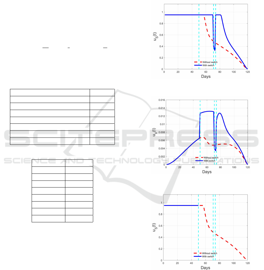
Figure 3: Optimal switching control u

(t) (solid blue line)

compared with a non switching solution (dashed red line).

Figure 4: Optimal switching control u

(t) (solid blue line)

compared with a non switching solution (dashed red line).

Figure 5: Optimal switching control u

(t) over the ﬁrst time

interval (solid blue line) and the remaining part without

switch (dashed red line).

The resulting optimal switching controls are plot-

ted in Figures 3 and 4 for u

(t) and u

(t) respectively,

while the sequences of control segments computed in

the iterative procedure are reported in Figures 5–8 for

ICINCO 2022 - 19th International Conference on Informatics in Control, Automation and Robotics

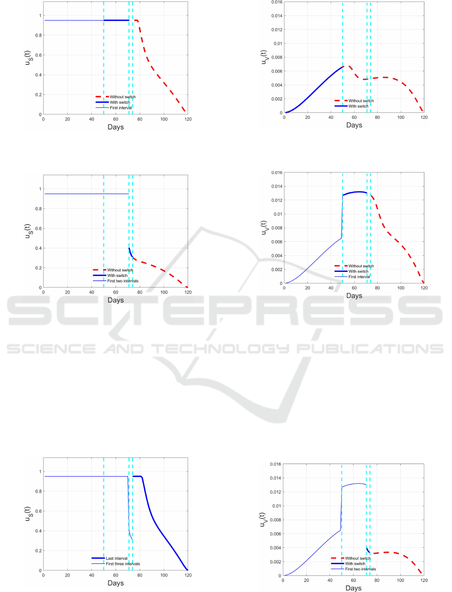
Figure 6: Optimal switching control u

(t) over the ﬁrst two

time intervals (thin and thick solid blue line) and the re-

maining part without switch (dashed red line).

Figure 7: Optimal switching control u

(t) over the ﬁrst

three time intervals (thin and thick solid blue line) and the

remaining part without switch (dashed red line).

(t) and in Figures 9 for u

(t).

The control design procedure is reported step by

step. In Figures 3 and 4 the full optimal controls are

reported as solid blue lines, showing the time switch

instants (

) = (50,71,74). In the same ﬁgure,

the switching solution is compared with the optimal

one obtained keeping the weights W

and W

constant

over all the integration (dashed red lines).

The above described iterative procedure is put in

Figure 8: Optimal switching control u

(t): thin solid blue

line for the already computed segments, thick solid blue

line) for the last segment.

Figure 9: Optimal switching control u

(t) over the ﬁrst

time interval (solid blue line) and the remaining part with-

out switch (dashed red line).

Figure 10: Optimal switching control u

(t) over the ﬁrst

two time intervals (thin and thick solid blue line) and the

remaining part without switch (dashed red line).

evidence by the sequences of picture. Starting from

Figures 5 and 9, the solutions of the ﬁrst optimal prob-

lem are reported and the corresponding evolutions for

I(t) and I

(t) are depicted in Figures 13 and Figures

17. They correspond to the ﬁnal optimal solution

for the time interval [0,50), evidenced in the Figures,

since at time

= 50 a switch occurs due to the pas-

sage of I

(t) from one region to the one above. The

red dashed lines in these ﬁgures represent the evolu-

tion if the switch were not applied. Actually, with the

Figure 11: Optimal switching control u

(t) over the ﬁrst

three time intervals (thin and thick solid blue line) and the

remaining part without switch (dashed red line).

Optimal Social Limitation Reduction under Vaccination and Booster Doses

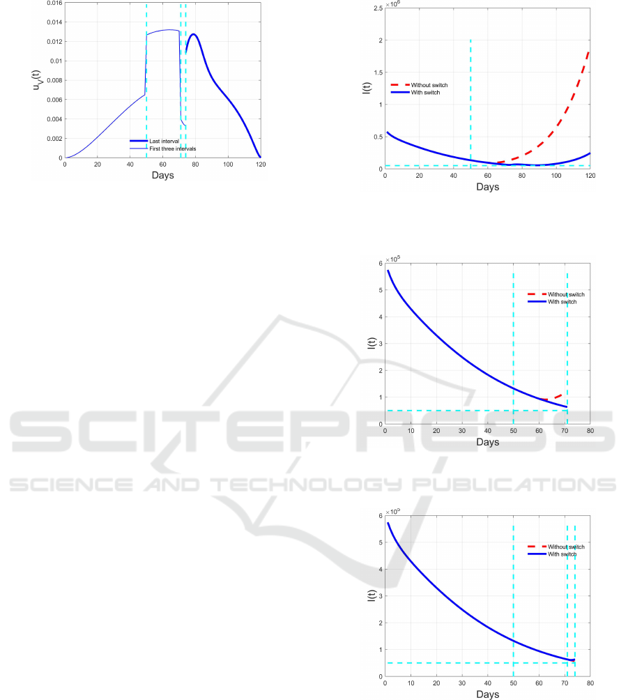
Figure 12: Optimal switching control u

(t): thin solid blue

line for the already computed segments, thick solid blue

line) for the last segment.

change of region, the new optimal problem is solved

with different weights for the controls, in particular

smaller than in the previous case due to the more dan-

gerous situation of a greater number of infected indi-

viduals above the ﬁxed threshold.

Figures 6 and 10 show the result of this latter

problem, with the new optimal control depicted from

t = 50 to the end. The segment computed in the pre-

vious step is marked with a thin blue line, the present

segment with a thick blue line and the red dashed line

denotes the remaining part of the solution if a new

switch were not present. The corresponding effect on

the optimal state evolution is reported in Figures 14

and 18 for the two classes of infected individuals. It

can be noted that the introduction of changes in the

weights of the cost function allow to react to a worse

situation with a greater control effort.

At time

= 74 the higher control action brings

the state variable I

(t) to return into the previous, less

dangerous, region of decomposition, so giving a new

switch with a consequent increment of the weights

for the control in the cost function. The segment of

controls in the time interval [

) = [71,74) are evi-

denced by thick blue solid curves in Figures 7 and 11

(t) and u

(t) respectively), while the correspond-

ing evolutions of I(t) and I

(t) are reported in Figures

15 and 19, with the same notation as for the previ-

ous segment. The reduction of the controls effort after

produces an increment of infected individuals once

more. This brings to a new switch in t =

and the

consequent evolution over the last time segment con-

sidered. Figures 8 and 12 report the evolution in such

a time interval for the controls, while Figure 16 and 20

depict the resulting time histories for I(t) and I

(t).

6 CONCLUSIONS

In the present paper an optimal control approach with

an available effort planned on the basis of the danger-

Figure 13: I(t) evolution under optimal switching control

(blue solid line) compared with the non switching solution

(red dashed line).

Figure 14: Switching (blue solid line) and non switching

(red dashed line) evolution of I(t) during the ﬁrst two time

intervals of the algorithm [0,50) and [50,71).

Figure 15: Comparison between switching (blue solid line)

and non switching (red dashed line) evolution of I(t) during

the third time interval [71,74).

ousness of the health conditions is proposed for deﬁn-

ing the individual and social contact limitations after

vaccination in COVID-19 pandemic situation. The re-

sults show how the possibility of allowing a greater,

even more expensive, effort in some severe conditions

while planning a reduction under less serious situa-

tions allow to have effective results with a global con-

ICINCO 2022 - 19th International Conference on Informatics in Control, Automation and Robotics

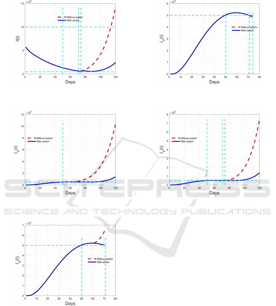
Figure 16: Comparison between switching (blue solid line)

and non switching (red dashed line) evolution of I(t) during

the fourth time interval [74,120).

Figure 17: I

(t) evolution under optimal switching control

(blue solid line) compared with the non switching solution

(red dashed line).

Figure 18: Switching (blue solid line) and non switching

(red dashed line) evolution of I

(t) during the ﬁrst two time

intervals of the algorithm [0,50) and [50,71).

tainment of the resources and the costs. In particular,

it has been shown how the restrictions on vaccinated

and not vaccinated individuals would have been dis-

tinguished, reducing them for vaccinated ones since

the beginning of the vaccination campaign. Actually,

the use of speciﬁc certiﬁcations for entering restau-

rants, theatres and, generally, attending public events

Figure 19: Comparison between switching (blue solid line)

and non switching (red dashed line) evolution of I

(t) dur-

ing the third time interval [71,74).

Figure 20: Comparison between switching (blue solid line)

and non switching (red dashed line) evolution of I(t) during

the fourth time interval [74,120).

with high number of participants, adopted in many

countries, is supported by these results.

REFERENCES

Dan, J. M., Mateus, J., Kato, Y., Hastie, K., Yu, E. D., and

Faliti, C. E. (2021). Immunological memory to sars-

cov-2 assessed for up to 8 months after infection. Sci-

ence, 371(6529):1–15.

Di Giamberardino, P. and Iacoviello, D. (2017). Optimal

control of SIR epidemic model with state dependent

switching cost index. Biomedical Signal Processing

and Control, 31.

Di Giamberardino, P. and Iacoviello, D. (2020). A control

based mathematical model for the evaluation of inter-

vention line in epidemic spreads without vaccination:

the covid-19 case study. Submitted to IEEE Journal of

Biomedical and Health Informatics.

Di Giamberardino, P. and Iacoviello, D. (2021). Evaluation

of the effect of different policies in the containment of

epidemic spreads for the COVID-19 case. Biomedical

signal processing and control, 65(102325):1–15.

Optimal Social Limitation Reduction under Vaccination and Booster Doses

Di Giamberardino, P., Iacoviello, D., F.Papa, and

C.Sinisgalli (2021). Dynamical evolution of COVID-

19 in Italy with an evaluation of the size of the

asymptomatic infective population. IEEE Journal

of Biomedical and Health Informatics, 25(4):1326–

1332.

Diagne, M. L., Rwezaura, H., Tchoumi, S. Y., and

Tchuenche, J. M. (2021). A mathematical model

of covid-19 with vaccination and treatment. Com-

putational and Mathematical Methods in Medicine,

(1250129):1–16.

Giordano, G., Blanchini, F., Bruno, R., Colaneri, P., Fil-

ippo, A. D., and Colaneri, M. (2020). Modeling the

COVID-19 epidemic and implementation of popula-

tion wide interventions in Italy. Nature Medicine, 26.

Liu, Z., Omayrat, M., and Stursberg, O. (2021). A study

on model-based optimization of vaccination strategies

against epidemic virus spread. In Proceedings of the

18th International Conference on Informatics in Con-

trol, Automation and Robotics - ICINCO,, pages 630–

637. INSTICC, SciTePress.

Olivares, A. and Staffetti, E. (2021). Optimal control-

based vaccination and testing strategies for covid-

19. Computer Methods and Programs in Biomedicine,

211(106411):1–9.

Radulescu, A., Williams, C., and Cavanagh, K. (2020).

Management strategies in a SEIR-type model of

COVID-19 community spread. Nature. Scientiﬁc Re-

ports, 21256.

Silva, C. J., Cruz, C., Torres, D. F. M., Munuzuri, A. P.,

Carballosa, A., Area, I., Nieto, J. J., Pinto, R. F., Pas-

sadouro, R., dos Santos, E., Abreu, W., and Mira, J.

(2021). Optimal control of the covid-19 pandemic:

controlled sanitary deconﬁnement in portugal. Scien-

tiﬁc Reports, 11(3451):1–15.

Tang, B., Bragazzi, N. L., Li, Q., Tang, S., Xiao, Y., and Wu,

J. (2020). An updated estimation of the risk of trans-

mission of the novel coronavirus (2019-nCov). Infec-

tious disease modeling, 5.

Van Den Driessche, P. (2017). Reproduction numbers of

infectious disease models. Infectious disease models,

2:288–303.

ICINCO 2022 - 19th International Conference on Informatics in Control, Automation and Robotics