Analyzing Cross-impact Matrices for Managerial Decision-making

Problems with the DEMATEL Approach

Shailesh Tripathi, Nadine Bachmann, Manuel Brunner and Herbert Jodlbauer

University of Applied Sciences Upper Austria Wehrgrabengasse 1-3, 4400 Steyr, Austria

Keywords: Cross Impact Analysis, Influence-Dependency Chart, Impact Matrix, Sensitivity Model, Active Sum, Passive

Sum, Decision Support System, Business Analytics, DEMATEL.

Abstract: Cross-impact matrices define pairwise direct impacts between variables representing the complexity of

various social, economic and technological systems. Business and management-related research primarily

utilizes the row and column sums of direct impact matrices to identify critical, influential, dependent, neuter,

and inert variables. However, the impact of drivers and outcomes in complex systems is usually difficult to

interpret accurately without considering the indirect impact of variables. This paper considers all impacts of

direct and indirect impact paths (known as the total impacts) between variables using the decision-making

trial and evaluation laboratory (DEMATEL) approach for direct impact matrices in which the rank order

remains stable (i.e., a stable equilibrium state exists). Numerical experiments show that the rank order of

variables and their role (influence or dependence) can change significantly when considering total impacts

between variables compared with when considering direct impacts only. This analysis can be used to support

management in strategic planning and decision-making, e.g., in an international business environment:

Management should attempt to obtain the total impacts matrix defining all direct and indirect impacts that

determine the rank order on which informed decisions are subsequently based. The results presented in this

paper indicate that impact paths between variables should be incorporated into the system with an in-depth

domain understanding. This enables the realistic capture of impacts and the establishment of a stable state for

obtaining an unbiased understanding of the roles of variables.

INTRODUCTION

As decision-makers, managers are faced with

strategic challenges when projects and processes are

affected by factors representing the complexity of

interdependence in business model innovation,

product innovation, strategy development, or

reorganization, as these factors are usually difficult to

understand and interpret. Cross-impact methods are

commonly used as analysis and decision support tools

in such cases. When few statistical or empirical data

are available, these methods enable theory-driven and

expert-oriented systems modeling (Panula-Ontto &

Piirainen 2018; Weimer-Jehle, 2006). Expert

judgments are processed and synthesized in a

systematic, formalized, and structured manner, with

the aim of identifying both direct and indirect impacts

between identified variables (Asan et al. 2004). In

contrast to the widespread use of direct impact

matrices in the cross-impact approach, few studies

(Arcade et al., 1999; Zimmermann & Eber, 2014;

Jodlbauer, 2020; Jodlbauer et al., 2021) have

addressed powered impact matrices.

This study investigates the cross-impact approach of

using the total impact matrix, which considers all

direct and indirect impacts from a given direct impact

matrix obtained by the decision-making trial and

evaluation laboratory (DEMATEL) approach (Gabus

& Fontela, 1972). This study draws on Gordon and

Hayward’s (1968) cross-impact approach, Vester and

Hesler’s (1982) sensitivity model, and Godet’s (1987)

MICMAC method. We present an analysis based on

simulated matrices of different orders that remain

stable when all direct and indirect impacts are

considered. Numerical experiments show that the

rank order of variables in the total impact matrix, as

compared with the direct impact matrix, can change

significantly depending on their categorization into

influential and dependent variables. This study

attempts to present a numerical analysis method that

can assist management in strategic planning by

emphasizing the importance of using the total impact

370

Tripathi, S., Bachmann, N., Brunner, M. and Jodlbauer, H.

Analyzing Cross-impact Matrices for Managerial Decision-making Problems with the DEMATEL Approach.

DOI: 10.5220/0011274600003269

In Proceedings of the 11th International Conference on Data Science, Technology and Applications (DATA 2022), pages 370-382

ISBN: 978-989-758-583-8; ISSN: 2184-285X

matrix for decision-making. In addition, it lays the

foundation for future empirical research that applies

the proposed method in practice. The following

sections provide an overview of cross-impact

analysis, discuss the current state of research, and

present the research questions.

1.1 Cross-impact Analysis

Based on direct impact matrices, Gordon and

Hayward (1968) introduced the cross-impact

approach. The model starts with the definition of the

relevant variables 



,



,…,



. According to Vester

and Hesler (1982), the pairwise influence between the

variables is coded using values of 0, 1, 2, or 3:

0 has a negligible impact on

1 has a small impact on

2 has a proportional impact on

3 has a great impact on











(1)

In general, the influence is not commutative, i.e.,

. The influence values are summarized in

the so-called direct impact matrix

()

{}

1,...,

0,1, 2, 3

and

0 for all 1,...,

ain

=∈

(2)

The direct impact matrix describes the pairwise direct

impact between each pair of variables, and can be

interpreted as the adjacency matrix of the weighted

direct graph describing the pairwise direct impact

between the variables (nodes of the graph). For

further analysis, the active sum (AS), passive sum

(PS), Q-value, and P-value are defined as follows

(Godet & Roubelat, 1996):

active sum

(sum of the row of the matrix )

passive sum

(sum of the column of the matrix )

-value

(quotient active sum over passive sum)

iik

jkj

ith

AS a

ith A

jth

PS a

th A

ithQ

PASP

−



-value

(product active sum by passive sum)

ithP

−

(3)

AS can be interpreted as the weighted outdegree of the

−ℎ variable (node), whereas PS refers to the

weighted indegree of the −ℎ variable (node). A

variable with a high AS value has a significant impact

on all other variables, and vice versa. A variable with

a high PS value is strongly influenced by the other

variables, and vice versa. The  -value reflects these

categories, as the variable with the highest  -value

has the greatest overall impact on the other variables,

i.e., it is the most active variable, while the variable

with the smallest  -value is most dependent on the

other variables, i.e., it is the most passive variable.

Active variables can be used to control or improve the

system. It is important to be able to manage active

variables, otherwise there is a risk of losing control of

the system. Passive variables can be considered as

output variables that measure success.

The  -value provides a measure of relevance. A

variable with a high  -value has a great impact on

the other variables and is strongly influenced by them.

Variables with high  -values are referred to as

critical variables and require the highest level of

management attention. Critical variables and their

relationships have to be understood to ensure the

successful configuration and management of the

system. Variables with small  -values are called

inert variables and should not be the focus of

management. In the so-called influence–dependency

chart (Godet and Roubelat, 1996), the system,

variables, and their relationships or significance can

be visualized (see Figure 1). The x- and y-axes of the

influence–dependency chart represent the passive

sum and the active sum of the variables, respectively.

Figure 1: Influence-dependency chart.

The influence–dependency chart and

distinguished between five categories of variables:

critical, influential, dependent, neuter, and inert. The

critical variables are those at or near the upper-right

corner. Critical variables are affected by and impact

many other variables. They are the most important

variables to be considered and can be expressed as

stake variables. Influential variables are located at or

near the upper-left corner. These variables influence

many other variables in the system, but are relatively

less affected by other variables. They can be

expressed as determinant variables. Dependent

variables are positioned at or near the bottom-right

corner. Dependent variables are more affected by the

,,ij ji

aa≠

Analyzing Cross-impact Matrices for Managerial Decision-making Problems with the DEMATEL Approach

371

system than they affect it. They can be expressed as

result variables to be monitored. Inert variables are

located at or near the bottom-left corner. These have

little influence on and low dependency on other

variables. They are relatively unconnected to the

system and can therefore be excluded from the impact

matrix. Neuter variables are averagely influential

and/or dependent variables. Nothing definite can be

said about them. A similar division of variables can

be found in Linss and Fried (2010), who use

categories of reactive, critical, inert, and active.

To illustrate the cross impact analysis method, an

example based on Vester (2000) is presented. For

better comprehensibility, only the first four variables

regarding urban development are utilized:

attractiveness for recreation

(





)

, need for leisure

facilities

(





)

, frequent use of open spaces

(





)

, and

variety of plant species

(





)

. The relationships

between these variables can be shown by a directed

weighted graph called an effect–cause diagram (see

Figure 2), or equivalently by the direct impact matrix

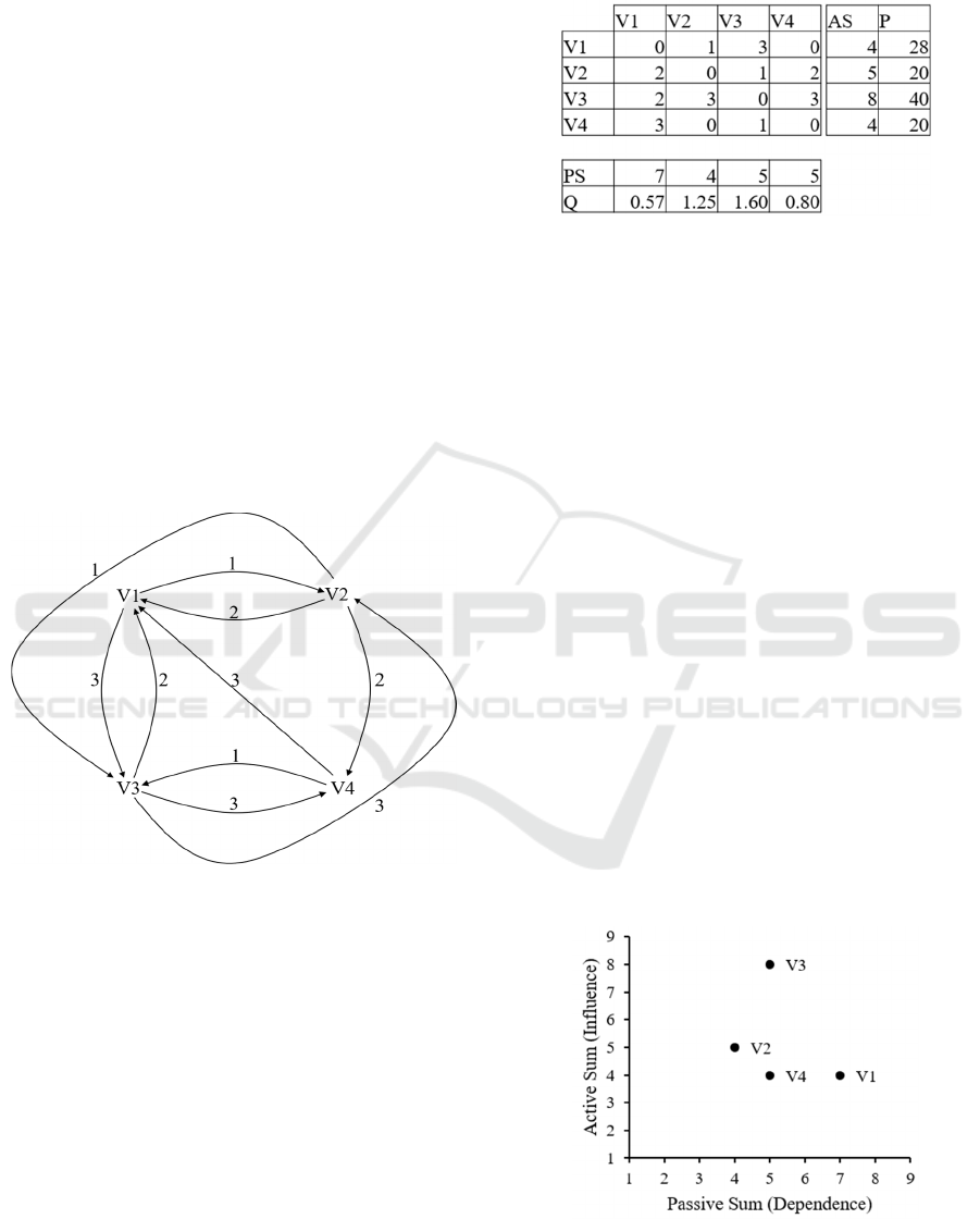
(see Table 1).

Figure 2: Effect-cause-diagram for the simple example.

Figure 2 shows the effect–cause diagram

(weighted directed graph) for the first four variables

discussed in Vester (2000). Table 1 presents all

pairwise impacts, AS values, PS values,  -values,

and  -values. Figure 3 illustrates the four variables

in the influence-dependency chart. Variable 



has

the highest AS and the highest  -value (i.e., the

highest impact on all other variables), as well as the

highest  -value (i.e., most critical variable). Variable





has the smallest  -value as well as the highest PS

(i.e., influenced the most by all other variables). 



and 



both have the smallest  -value (i.e., most inert

variables).

Table 1: Corresponding impact matrix for the simple

example.

There are many other models similar to Vester’s

sensitivity method (Vester & Hesler, 1982). The

analysis of several scenarios by Gausemeier et al.

(2001) is based on an impact matrix with the same

structure as Vester’s impact matrix:



Vester

=

,



,...,

,...,

∈



0,1,2,3





and



,

=0 for all =1,..., (4)

The cross-impact approach (Gordon & Hayward,

1968) utilizes a transfer matrix describing the

pairwise probability of the occurrence of an event that

is dependent on another event:



cross impact

=

,



,...,

,...,

∈



0,1

]



and



,

=0 for all =1,..., (5)

Godet (1987; 2000) developed a scenario analysis

whereby the structural analysis uses the impact matrix



Godet

=

,



,...,

,...,

∈



0,1





and



,

=0 for all =1,..., (6)

It does not matter which coding the weighting has—

as long as 

,

≥0 and 

,

=0, the model developed

in section 2 is applicable.

Figure 3: Corresponding influence-dependency chart for

the simple example.

DATA 2022 - 11th International Conference on Data Science, Technology and Applications

372

1.2 State of Research and Research

Questions

The various applications of the cross-impact

approach or similar methods cover different areas

such as social network analysis (Wasserman & Faust,

1994), international business networks (Bolívar et al.,

2019; Caraiani, 2013; Ho & Chiu, 2013; Joseph et al.,

2014), project management (Frahm & Rahebi, 2021;

Reiss, 2013), scenario analysis (Bañuls & Salmeron,

2007; Bañuls & Turoff 2011; Medina et al., 2015),

and strategic management (Alizadeh et al., 2016).

Based on the adjacency matrix for weighted

directed graphs, Wasserman and Faust (1994)

investigated social networks. Following the so-called

“sociomatrices” of Wasserman and Faust (1994), Ho

& Chiu (2013) filtered more than 20,000 patents and

created a network of patent activities and knowledge

flows among 30 semiconductor companies. Caraiani

(2013) derived a complex network based on a

Granger causality matrix of relationships between

countries, allowing them to characterize international

business cycles. Joseph et al. (2014) applied a so-

called multiple linear regression (MLR)-fit network

(MLR combined with big data and network science)

to model global economic interactions, providing an

accurate phenomenological description with high

predictive power despite the large number of possible

interaction channels. Global foreign direct investment

networks were analyzed by Bolívar et al. (2019), who

prepared a directed network matrix covering 229

countries for each year.

The cross-impact approach has been applied in

project management to contribute to stakeholder

management for mega projects (Frahm & Rahebi,

2021) and to model all project stakeholders and their

relationships (Reiss, 2013). Scenario analysis has

been used to assess national technology policies

(Bañuls & Salmeron, 2007; Bañuls & Turoff 2011),

identify the barriers that influence decisions to invest

in solar power (Medina et al., 2015), and develop

more resilient conservation policies in the energy

industries (Alizadeh et al., 2016).

Other diverse applications relate to the

investigation of sustainable development strategies

using the sensitivity model (Chan & Huang, 2004;

Huang et al., 2009), the combination of cross-impact

analyses with patent analyses to estimate

technological impacts based on multiple patent

classifications (Choi et al., 2007), the analysis of the

potential for telemedicine (Gausemeier et al., 2012),

as well as the development and analysis of key

performance indicators for organizational structures

in construction, real estate management

(Zimmermann & Eber, 2014), and production

(Köchling et al., 2018). Dubey and Ali (2014)

employed a fuzzy cross-impact analysis approach to

identify flexible manufacturing system dimensions

and their interrelationships. Asan et al. (2004)

presented a qualitative cross-impact analysis in terms

of fuzzy relationships. The analytic hierarchy process

(AHP) decision model has been combined with

cross-impact analysis as a technological forecasting

approach by Cho and Kwon (2004) and Saaty (2004).

Barati et al. (2019) presented an integrated method

that combines AHP techniques with cross-impact

analysis to identify important strategic factors in

agriculture.

In most of the papers on the cross-impact

approach, the direct impact matrix is used to

determine AS and PS. Relatively few authors have

addressed powered impact matrices (Arcade et al.,

1999; Jodlbauer, 2020; Zimmermann & Eber, 2014).

The direct impact matrix shows the direct pairwise

impact between two variables 



and 



. In

comparison, the squared impact matrix shows the

indirect impact of variable 



on variable 



via

exactly one intermediate variable. The squared

impact matrix refers to all indirect connections with

path length two i.e., one intermediate variable (node).

Generally, the −ℎ power of the impact matrix

describes the indirect pairwise impact between the

variables via all possible paths with length , i.e., −

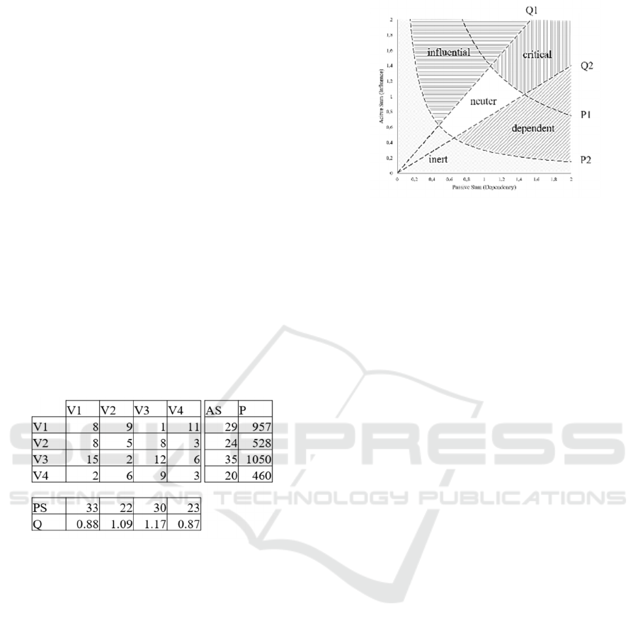
1 intermediate variables. For illustration, the squared

impact matrix is shown for the simple example

mentioned above (see Table 2):

=

0130

2012

2303

3010

,



=

89111

8583

152126

2693



(7)

Godet (1987) introduced the MICMAC (Impact

Matrix Cross-Reference Multiplication Applied to a

Classification: Matrices d’Impacts Croises—

Multiplication Appliqué un Classement) method to

analyze the indirect relationships and diffusion of

impacts through paths and loops involving

intermediate variables. Godet defined both the

influence and the dependence rank. The influence

rank is based on the AS value (row sum) of the impact

matrix. The variable with the highest AS has influence

rank 1, the variable with the second-highest AS has

influence rank 2, and so on. The dependence rank is

based on the PS value (column sum). The variable

with the highest PS is assigned dependence rank 1,

and so on. Indirect classification is obtained by

increasing the power of the impact matrix and

determining the row and column sums of the powered

matrices. According to Coates and Godet (1994), the

Analyzing Cross-impact Matrices for Managerial Decision-making Problems with the DEMATEL Approach

373

classification, especially the rank order, generally

becomes stable for power degrees higher than 5. Our

research contribution builds on precisely this point,

first, by identifying counter examples, second, by

demonstrating analytically that there are cases in

which no stable state exists, and third, by deriving an

analytical categorization of the direct impact matrix

that leads to stable rank orders. Linss and Fried

(2010) presented an advanced impact analysis

technique for processing data from cross-impact

analyses considering both direct and indirect impacts.

They examined manually calculated matrix

multiplications and then evaluated the stability of

sequences of active or passive sums. Gräßler et al.

(2019) modeled the indirect impacts by applying the

page-rank algorithm (Page et al., 1999) to the

corresponding adjacency matrix. The determined

page-ranks are then applied instead of the

aforementioned influence ranks when using powered

impact matrices. The dependency rank is determined

by the page-rank of the transposed impact matrix.

Table 2: Squared impact matrix with active sum, passive

sum,  -values, and  -values.

For a time-discrete Markov chain (Norris, 1998), the

transition matrix 



describes the transition

probability from one state to another. A Markov

transition matrix has some similarities to the impact

matrix introduced by Gordon and Hayward (1968),

but also some structurally different characteristics:





=

,



,...,

,...,

∈



0,1

]



and

∑



,





=1 for all j =1,..., (8)

The column sum (PS) for a Markov transition matrix

has to be equal to one for every column, and the

diagonal elements are not necessarily equal to zero.

Under certain assumptions, a Markov chain is stable

and converges to the unique invariant distribution



→











=

for every arbitrary initial state 



(9)

Figure 4: Influence-dependency chart and categorization

regions.

One of the main objectives of this paper is to

investigate the direct impact matrices for which the

total impact matrix is stable and convergent in the

sense of converging rank orders of P-values and Q-

values.

The research questions addressed in this article

are:

(i) How are variables ranked or how do their roles

change when total impact matrices are used

instead of the corresponding direct impact

matrices? To answer this question, we perform

comparisons between the direct impact matrix

and the total impact matrix (sum of direct and all

indirect impacts) of matrices of different orders

to identify changes in the drivers and outcomes

(influence–dependence).

(ii) How do transitive relations affect the ranking of

variables? To answer this question, the

influence of transitive relations on the total

impact matrices compared to their direct impact

matrices is analyzed.

(iii) What are the implications of applying the total

impact matrix for managerial decision-making?

Jodlbauer et al. (2021) discussed the conditions

under which normalization occurs, i.e., the  -value

and the rank orders of the powered impact matrices

converge to a stable state. Furthermore, the rank

orders of  -values, AS, and PS converge to a stable

state. In the case of convergence, the stable state

matrix should be used to determine the AS, PS,

 -values, and  -values, and the influence–

dependency chart for their visualization.

The remainder of this article is organized as

follows. Section 2 provides a brief introduction to the

DEMATEL approach. For impact matrices, the

DEMATEL model is applied to determine the total

impact matrix, which reflects all possible direct and

DATA 2022 - 11th International Conference on Data Science, Technology and Applications

374

indirect impacts between all variables, and to prepare

an influence–dependency chart and categorize the

variables. In section 3, numerical analysis is

conducted to identify the possible differences that

occur when using the direct impact matrix or the total

impact matrix. Finally, section 4 discusses the

implications of the proposed model for research and

management and identifies the limitations of this

study, and presents some ideas for future research.

INDIRECT IMPACT MODEL

(TOTAL IMPACT MATRIX)

We briefly describe the determination of the total

impact matrix using the classical DEMATEL

approach (Gabus & Fontela, 1972), the visualization

of the influence–dependency chart, and the

categorization of variables. Let =

,



,…,

,…,

∈

ℝ



be a direct impact square matrix with real

nonnegative entries 

,

≥0 and 

,

=0. The first

step is the normalization of the direct impact matrix,

which is defined as:

=







(10)

where

is defined as follows:

=



∑



,





,



∑



,





 (11)

=

,



,…,

,…,

∈ℝ



, and 0≤

,

≤1.

The total impact matrix is obtained by adding all

direct and indirect impacts:

()()

()

lim ,

assuming that a limit exists, we have:

lim lim

lim

The final total impact matrix is:

T D D DID ID D

T DID ID DID

TDID

→∞

−−

−

→∞ →∞

−−

→∞

−

==−−

=− −=−

=−





(12)

The matrix =

,



,…,

,…,

reflects all direct and

indirect impacts and is called the total impact matrix;

this is the sum of all powered normalized impact

matrices. To visualize the stable impact state and

categorize the variables, the AS, PS, -values, and

-values are determined for the stable state matrix 

and the influence–dependency chart is utilized for

matrix  (see Figure 4).

Figure 5: Spearman rank correlation 





(



)

,

(



)

 and







(



)

,

(



)

 between  -values and  -values with

respect to the number of non-zero entries of randomly

generated matrices.

active sum

(sum of the row of the matrix )

passive sum

(sum of the column of the matrix )

-value

(quotient active sum over passive sum)

iik

jkj

iii

AS t

PS t

PASPS



-value

(product active sum by passive sum)

(13)

The AS, PS, -values, and  -values are used to

construct the influence–dependency chart shown in

Figure 4. The x-axis of the influence–dependency

chart reflects the PS values and the y-axis reflects the

AS values. We define ISO-P-curves, 



(),

and ISO-Q-curves, 



(), as functions of 

as follows:





(



)









()= 

(14)

An ISO-P-curve for a fixed  -value is a decreasing

function containing all pairs

(

,

)

that have the

same  -value. The ISO-P-curve for a fixed -value

consists of all pairs that have the same relevance  for

Analyzing Cross-impact Matrices for Managerial Decision-making Problems with the DEMATEL Approach

375

the system. An ISO-Q-curve for a fixed  -value is an

increasing function of pairs

(

,

)

that have the

same power  to influence the system or to be

controlled by the system. On the 45° line where





(



)

=, there is an equilibrium between

influential and dependent categories.

For the five categories addressed in Figure 4—

critical, influential, dependent, neuter, and inert—we

propose the following definitions:

()

, with:

and,

belong to

critical 2 1 and P P1

influential 1 and P P2

dependent 2 and P P2

neuter 2 1 and P2 P P1

inert P P2

PS AS

PPSAS

QQQ

⇔≤≤ ≥

⇔> ≥

⇔< ≥

⇔≤≤ ≤<

⇔<

(15)

For practical reasons, the -values 1 and 2 and the

 -values 1 and 2 can be chosen to ensure that the

number of essential variables (critical, influential, and

dependent) is manageable. Let 



be the number

of manageable critical variables, 



be the

number of manageable influential variables (input),





be the number of manageable dependent

variables (output), and 



be the number of

intended inert variables. For these values ( being the

total number of variables and 



being the total

number of intended neuter variables), the following is

true:

>0,



>0,



>0,



>0,





>0,







+



+



+



+



=

2<1<1,2<1 (16)

To prioritize management activities, we propose the

following setting to place the focus on the most

important issues, that is, the management of key

variables (i.e., critical, influential, and dependent

variables). Fix 



,



,



 



and use the following criteria:

(



)

Choose 2:



(

, 

)

∈

 <2



=



(



)

Choose 1:



(

, 

)

∈





>1   ≥2=



(



)

Choose 2:



(

, 

)

∈





<2   ≥2=



(



)

Choose 1:



(

, 

)

∈2≤





≤1   ≥1

=



whereby,

=



(





,



=1,2,… ,



(17)

The output variables should be mainly used to

monitor the system and the input variables should be

used to control the system. If an input variable is

mainly controlled by external stakeholders, there is a

high risk that the system is not manageable. The

critical variables require the greatest attention from

management, who must monitor and control all

critical variables.

NUMERICAL ANALYSIS

Numerical analyses of randomly generated direct

impact matrices are now presented to illustrate the

importance of the total impact matrix

and its

comparison with the direct impact matrix

. For the

analysis, the following tasks must be performed:

1. Generate random direct impact matrices  of

order  (variables) by varying nonzero entries of

 such that the row sum and column sum of each

variable are greater than zero. We generate

direct impact matrices of order =

20,30,40,50,60,80 and 100 with different

proportions of nonzero entries varying from

0.05,0.1,0.15,…,1 to analyze the effect of

higher-order matrices and transitive relations of

the total impact matrix. For random matrix

generation, we start with a null matrix  of order

, and assign nonzero entries (direct impacts)

sampled uniformly from {1,2,3} to m

nondiagonal entries of 

(

≥, and ≤





−

)

2. Compare the influence–dependence measures

between direct impact matrices  and

corresponding total impact matrices .

Calculate the influence–dependence measures

(

,,, and 

)

and compare the  -values

and  -values between matrices  and  by

computing the Spearman rank correlation

(Spearman, 1904) to show the differences

between the ranks of variables with respect to

the number of nonzero entries in matrix 

3. Compute the proportion of variables that change

from influential to dependent and vice versa by

DATA 2022 - 11th International Conference on Data Science, Technology and Applications

376

examining 

(



)

and 

(



)

values of variables

considering different values for 1 and 2 (see

Figure 4).

4. Determine the impact of the transitive relations

of variables on the total impact matrix.

For the numerical analysis, ∼600,000 random

matrices were generated by varying the number of

nonzero entries in direct impact matrices of order .

Next, the matrices were analyzed to evaluate the rank

difference of variables, where the ranks of variables

were computed from the direct impact matrices  and

corresponding total impact matrices . The Spearman

rank correlation







(



)

,

(



)

,





(



)

,

(



)



between the P-values and -values of each direct

impact matrix and corresponding total impact matrix

was calculated to summarize the rank difference of

variables of randomly generated direct impact

matrices. The results are shown in Figure 5. The

x-axis is the number of nonzero entries in the

randomly generated matrices. The y-axis is the

Spearman rank correlation







(



)

,

(



)

,





(



)

,

(



)

 of -values and

-values, summarizing the rank difference of

variables. The Spearman rank correlation results

show that the total impact matrices  provide

different rankings of variables than the corresponding

direct impact matrices . The rank correlation

variation is higher in sparse matrices than in dense

matrices, indicating that the rank difference of

variables is likely to be higher in sparser matrices.

Next, the highest and lowest rank correlation of

 -values and  -values were computed (see Figure

5). The highest and lowest correlations for  are

~0.99 (when, for instance, matrix  has 228 nonzero

entries) and 0.62 (when matrix  has 34 nonzero

entries). The highest and lowest correlations for  are

~0.99 (when, for instance, matrix  has 228 nonzero

entries) and ~0.66 (when matrix  has 32 nonzero

entries). The highest rank correlation values indicate

that the ranking of variables has not changed

significantly and the same rank is maintained in both

matrices for  and . The lowest rank correlation

values show that the ranking of variables obtained

using the total impact matrix  has changed

significantly. A significant change in ranking means

that the influence–dependence effect of variables on

each other calculated by the direct impact matrix  is

significantly different from that given by the total

impact matrix . Further, the rank difference for

matrices varies between the minimum and maximum

values.

In other cases, variables may change from

influential to dependent or from dependent to

influential in the total impact matrix  compared with

the direct impact matrix , defined as a role-change.

For this analysis, we calculated the proportion of role-

change variables in the total impact matrix as follows.

We selected different values for 1 and 2 as

decision boundaries to determine whether 



(



)

and





(



)

for the 



variable are on the same side of the

decision boundary (i.e., 



(



)

>1∧



(



)

>1

or 



(



)

<1∧



(



)

<1), which defines the

influence or dependence effect of the variable. The

selected decision boundaries 1 and 2 were {(1,1),

(1.05, 0.95), (1.10, 0.90), (1.15, 0.85), (1.20, 0.80),

(1.25, 0.75)}. If a variable does not lie on the same

side of the decision boundary for both the direct

impact matrix and total impact matrix, then the role

of this variable as an influential or dependent variable

is different in the total impact matrix than in the direct

impact matrix. The proportion was calculated as

follows:

()

() ()

()

() ()

()

21 12

ii ii

IQA Q QT Q QA Q QT Q

prp D T

<∧ > ∨ >∧ <



(18)

where 

(

)

is an indicator function that returns 1 if the

input is true and 0 otherwise;

is the order of the

matrix. We further estimated the percentage of

matrices that have role-change variables when using

the total impact matrix compared with the direct

impact matrix for randomly generated matrices of

order =20,30,40,50,60,80 and 100. The results

are presented in Table 3. The first column is the

interval of the percentage of role-change variables in

a total impact matrix

(



)

compared with a direct

impact matrix

(



)

. The other columns show the

percentages of randomly generated matrices in

corresponding role-change intervals for different

boundaries of 1 and 2. The role-change categories

of variables are divided into four intervals to better

understand the likelihood of matrices that have no

change, small change, medium change, or large

change in the influence–dependence groups of

variables in  compared with . The four intervals

are: 1) no change, i.e., equal to zero, 2) small change,

i.e., (0,5]% of variables change role, 3) medium

change, i.e., (5,10]% of variables change role, and 4)

large change, i.e., >10% of variables change role.

Analyzing Cross-impact Matrices for Managerial Decision-making Problems with the DEMATEL Approach

377

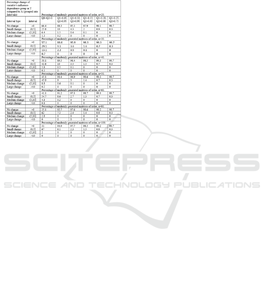
Table 3: Percentage of randomly generated matrices in

different role-change intervals in their total impact matrix

 compared to direct impact matrix A.

In Table 3, as the matrix order increases, the

percentage of matrices in the no change category

decreases for the cases where 1=2=1. In

addition, a significant percentage of matrices show a

small change, the percentage of matrices that show a

medium change varies from ~6.4% to 2%, and fewer

than 1% of matrices fall into the large change

category. As the width between decision boundaries

1 and 2 increases, the percentage of matrices in

the no change category increases from 80% to 99.7%.

Matrices gradually fall into the no change category as

the width between 1 and 2 increases, with only a

small fraction exhibiting small or medium change.

The percentage of matrices in the small change and

medium change categories decreases from 11.7% to

0.3% for different values of 1 and 2 (in increasing

order), and for different orders (n) of matrices.

However, we did not consider the change in neuter

variables to influence–dependence groups. This

analysis provides two important insights. First, it

highlights the importance of the total impact matrix,

as we observe that the matrices fall into the categories

of small, medium, and large change. Second, we can

see the importance of the selection of decision

boundaries 1 and 2. The user must select valid

impact boundary criteria under the supervision of

domain experts to determine 1 and 2; otherwise,

the indirect impact model will produce ineffective

results.

Next, the percentages of matrices in the four

different role-change categories based on the

proportion of nonzero entries in random direct impact

matrices of different orders were calculated. The

results are shown in Figure 6. More than 50% of the

sparser matrices (proportion of nonzero entries of

0.05–0.25) show a small, medium, or large change in

the influence–dependence groups of variables when

1=2=1

for different orders of matrices (see

Figure 6). As the matrices become dense, the rank

order difference decreases gradually, and the

percentages of matrices showing a small change in

influence–dependence groups of variables increase.

As the width increases between 1 and 2, the small,

medium, and large change categories disappear, and

a small fraction of the matrices remain in the small

and medium change categories.

It is important to note that the small change

(0,0.05] (interval (only some variables change role),

in which a significant percentage of matrices are

grouped (depending on the width between 1 and

Q2), is not trivial and should not be ignored. Domain

experts should assess the overall impact of these few

variables. Even if the number of variables that change

their group orders is small, the overall impact can be

large depending on the type of problem that is

addressed. Nevertheless, the change may be large or

small, which underscores the importance of a total

impact matrix from which influence–dependence

ranks can be calculated to measure the direct and

indirect impact of the variables. In this numerical

analysis, categorizing the variables that change

groups into these four categories highlights the

importance of the total impact matrix

for

measuring the indirect impacts of the variables on

each other.

Finally, we examined the effect of transitive

relations on the proportion of variables that changed

influence–dependence groups (role-change) in . We

searched for transitive relations using a weighted

transitive measure. A weighted transitive relation in

the direct impact matrix is defined as follows: in a

direct impact matrix, a triplet

(

,,

)

is transitive,

where

(

,

)

(

,

)

(

,

)

is a set of ordered pairs

defining the relations between the 



,



and 



variables, if the impact 

,

≥

,

,

,

 given

that 

,

,

,

>0. We applied the social network

analysis package sna (Butts, 2008) to calculate the

transitive measure for a randomly generated direct

impact matrix. The transitive measure is the fraction

of transitive relations for which 

,

≥

,

,

,



(Wasserman & Faust, 1994):

DATA 2022 - 11th International Conference on Data Science, Technology and Applications

378

()

,,,,,

111

min , 0 0

trn(A)

nnn

ik ij jk ij jk

ijk

jiki

nnn

ij jk

ijk

jiki

Ia a a a a

Ia a

===

≠≠

≠

===

≠≠

≠

≥∧≠∧≠

≠∧ ≠



(19)

The main objective of this analysis is to understand

whether changing the role of the variables in the

influence–dependence group in  produces a

systematic effect as the order of the matrices and the

number of transitive relationships change. A second

reason for this analysis is to understand the

importance of assigning impacts between variables

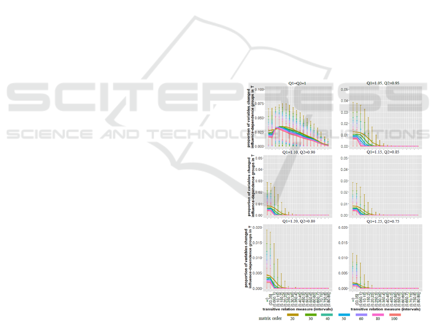
with transitive relations. The results of the average

change in proportion of variables with respect to the

transitivity measure (divided into different intervals

in increasing order) are shown in Figure 7 for

matrices of different orders and with different

decision boundaries 1 and 2. The results for 1=

2=1 show that an average of ~2.5% of variables

change their role in the influence–dependence group

in  when no or a small number of transitive relations

are observed. This value decreases gradually as the

number of transitive relations increases. When the

decision boundary threshold for 1 and 2 is

changed, the expected proportion of variables that

change the influence–dependence group in 

decreases and the expected proportion is

insignificant. This trend remains similar for matrices

Figure 6: Proportion of randomly generated matrices in

different role-change intervals with respect to the

proportion of non-zero entries in the randomly generated

matrices.

of different orders; however, there is a slight decrease

(downward shift) in the average proportion change of

variables as the order of the matrices increases,

indicating that the average percentage change in each

variable becomes smaller. The expected change

approaches zero in denser matrices (where the

number of transitive relations is higher) for all matrix

orders. The complexity of the relations between

variables (defined as the impact) may result in the

variables being grouped into different categories so as

not to ignore indirect impacts when using a direct

impact matrix for complex decision-making in a

business scenario. However, the total impact matrix

may be ineffective and redundant if impacts are added

arbitrarily without proper consideration, or if the 1

and 2 boundaries are not carefully selected.

Otherwise, the results could lead to inaccuracies and

produce an ineffective impact matrix, resulting in

incorrect calculations.

DISCUSSION AND

CONCLUSION

4.1 Research Implications

The following research implications arise from this

study. First, when the direct impact matrix  is very

sparse (i.e., contains few impacts), there is a high risk

that using direct impact matrix analysis to identify

influence–dependence variables will produce

incorrect results. Second, the numerical analysis

shows that the rank orders, importance, or category of

variables can change significantly between the direct

impact matrix  and the total impact matrix .

We observe two types of changes. First, a rank

change, where the role of the variables remains the

same. Second, a change in the influence–dependence

groups in the total impact matrix. Both types lead to

different interpretations of the system and variables

when using the total impact matrix . The proportion

of influence–dependence variables in the total impact

matrix  is significantly different for sparser

matrices. This affects whether decisions should be

made based on matrix  or matrix . A greater

number of transitive relations (high transitive score)

in the direct impact matrix  will result in a smaller

difference in the rank orders of variables between

matrix  and matrix , and so  does not provide any

significant results. When matrix  is sparse, the

difference in rank orders is greater.

In managerial applications, a higher number of

transitive relations may indicate one of three things,

Analyzing Cross-impact Matrices for Managerial Decision-making Problems with the DEMATEL Approach

379

assuming that for variables , , and , 

,

≥



,

,

,

 holds (as discussed in section 3): 1) A

direct impact with an in-depth domain understanding;

2) Inaccurate/arbitrarily assigned impacts; 3) A

relation derived by estimating indirect impacts. In the

second and third cases, the results of the total impact

matrix are useless or incorrect. It may seem that the

indirect relations are known, a direct impact matrix

analysis may be applicable, or a denser random

relation may lead to ineffective results. It is important

not to introduce impacts randomly and not to assign

indirect relations by establishing direct relations

between variables. Our analysis emphasizes that

indirect impacts should be computed for managerial

applications, assigning only direct impacts (using an

appropriate evaluation criterion) to construct an

initial direct impact matrix, and using a statistically

valid criterion with an appropriate domain

understanding for 1 and 2.

4.2 Managerial Implications

Systems that are difficult to understand and interpret

pose a strategic challenge to decision makers and

stakeholders. In decision making, for example, at the

top management level of a multinational company,

decision makers deal with systems that are difficult to

oversee and contain pairwise impacts of direct as well

as indirect variables. Our method makes the indirect

impact of variables visible and manageable: The

presented study can contribute to an improved

visualization (see influence-dependency chart of

matrix ) as well as to a better understanding of total

impact matrices compared to the use of direct impact

matrices, thus supporting consensus building among

decision makers and helping management in strategic

planning and decision-making processes (e.g.,

implementing targeted, well-coordinated actions).

Key variables can be identified and visualized in the

influence-dependency chart. The decision boundaries

in the influence-dependency chart should be selected

carefully so that the overall impact of the variables is

not over- or underestimated. In addition, management

can use the chart to determine whether variables in

the system are critical variables (and should thus be

treated with the greatest attention) or not. KPIs can be

derived from dependent output variables and support

management in decision-making.

The following recommendation can be made to

managers: The insight of a cross-impact analysis

conducted with the DEMATEL approach is that

significant differences between a direct impact matrix

and a total impact matrix are possible. However, there

might be cases where the ranking of variables does

not change when proportion of non-zero entries are

higher. This may be due to an arbitrary selection of

relations resulting in a high proportion of non-zero

relations, or unassessed transitive relations. If the

experts correctly assess the transitive relations, this

will not affect the interpretation of the results, but

random or incorrect assessment of the relations would

lead to misinterpretation and potentially provide

ineffective or redundant results. Therefore, managers

are recommended to always work with matrix  when

estimating the overall impact of variables on each

other, as the variables may have a different

categorization compared to the direct impact matrix

. In contrast to matrix , the total impact matrix 

also contains all indirect relationships between the

variables. The potential applications of the model are

diverse and extend far beyond the management level.

Especially in international business, when global

production networks, international operations

networks, networks of foreign suppliers, global FDI

networks, or global R&D networks are concerned, the

method can support decision makers in complex

decisions. Further application examples are business

model innovation, urban development, politics, or

risk analysis.

Figure 7: Average proportion of variables changed.

4.3 Future Research and Limitations

In future research, the presented DEMATEL model

should be applied to pilot projects, case studies, and

DATA 2022 - 11th International Conference on Data Science, Technology and Applications

380

empirical studies, taking into account the complexity

of the system’s transitive, modular, or hierarchical

relationships. The presented approach is applicable in

practical environments (e.g., production, quality

control, process optimization, business model

innovation) and not only in randomly generated

situations. One limitation of this study is that the

model has been exclusively applied to positive

matrices with the coding



1,2,3



. In the future, it is

recommended that investigations examine whether

the model can be applied to matrices with other

codings that allow negative values. A key challenge

to overcome is the definition of impacts between

variables, especially in transitive cases. For example,

in developing a direct impact matrix, different experts

may assign different impacts, leading to cases of

transitivity where indirect and direct impacts exist

between variables and the weights of the sums of

indirect and direct relations are different. Such cases

need to be investigated using cross-impact analysis

matrices that account for direct and indirect impacts.

Another challenge involves validating the impact of

variables in practical situations (allowing valid

interpretation by domain experts) using cross-impact

analysis matrices that consider direct and indirect

impacts of realistic business scenarios.

ACKNOWLEDGEMENTS

This paper is a part of X-pro project. The project is

financed by research subsidies granted by the

government of Upper Austria.

REFERENCES

Alizadeh, R., Lund, P. D., Beynaghi, A., Abolghasemi, M.,

& Maknoon, R. (2016). An integrated scenario-based

robust planning approach for foresight and strategic

management with application to energy industry.

Technological Forecasting and Social Change, 104,

162–171.

Arcade, J., Godet, M., Meunier, F., & Roubelat, F. (1999).

Structural analysis with the MICMAC method &

Actor's strategy with MACTOR method. In J. Glenn

(Ed.), Futures Research Methodology. American

Council for the United Nations University: The

Millennium Project.

Asan, U., Bozdağ, C. E., & Polat, S. (2004). A fuzzy

approach to qualitative cross impact analysis. Omega

32(6), 443–458.

Bañuls, V. A., & Salmeron, J. L. (2007). A scenario-based

assessment model—SBAM. Technological

Forecasting and Social Change 74(6), 750–762.

Bañuls, V. A., & Turoff, M. (2011). Scenario construction

via Delphi and cross-impact analysis. Technological

Forecasting and Social Change 78(9), 1579-1602.

Barati, A. A., Azadi, H., Dehghani Pour, M., Lebailly, P.,

& Qafori, M. (2019). Determining key agricultural

strategic factors using AHP-MICMAC. Sustainability

11(14), 3947.

Bolívar, L. M., Casanueva, C., & Castro, I. (2019). Global

foreign direct investment: A network perspective.

International Business Review, 28(4), 696-712.

Butts, C. T. (2008). Social network analysis with sna.

Journal of statistical software, 24(6), 1-51.

Chan, S. L., & Huang, S. L. (2004). A systems approach for

the development of a sustainable community—the

application of the sensitivity model (SM). Journal of

Environmental Management 72(3), 133–147.

Caraiani, P. (2013). Using complex networks to

characterize international business cycles. PloS one,

8(3), e58109.

Cho, K. T., & Kwon, C. S. (2004). Hierarchies with

dependence of technological alternatives: A cross-

impact hierarchy process. European Journal of

Operational Research 156(2), 420–432.

Choi, C., Kim, S., & Park, Y. (2007). A patent-based cross

impact analysis for quantitative estimation of

technological impact: The case of information and

communication technology. Technological Forecasting

and Social Change 74(8), 1296–1314.

Coates, J. F. P., & Godet, M. (1994). From anticipation to

action: a handbook of strategic prospective. Paris:

UNESCO Publishing.

Dubey, R., & Ali, S. S. (2014). Identification of flexible

manufacturing system dimensions and their

interrelationship using total interpretive structural

modelling and fuzzy MICMAC analysis. Global

Journal of Flexible Systems Management 15(2), 131–

143.

Frahm, M., & Rahebi, H. (2021). Management von Groß-

und Megaprojekten im Bauwesen. Wiesbaden: Springer

Vieweg.

Gabus, A., & Fontela, E. (1972). World problems, an

invitation to further thought within the framework of

DEMATEL. Battelle Geneva Research Center,

Geneva, Switzerland, 1-8.

Gausemeier, J., Ebbesmeyer, P., & Kallmeyer, F. (2001).

Produktinnovation Strategische Planung und

Entwicklung der Produkte von morgen. München:

Hanser.

Gausemeier, J., Grote, A. C., & Lehner, M. (2012).

Zukunftsmarkt Telemedizin—Anforderungen an die

Produkte und Dienstleistungen von morgen. In J.

Gausemeier (Ed.), Vorausschau und

Technologieplanung (Band 306). Paderborn: HNI-

Verlagsschriftenreihe.

Godet, M. (1987). Scenarios and strategic management.

London: Butterworths.

Godet, M. (2000). The art of scenarios and strategic

planning: tools and pitfalls. Technological Forecasting

and Social Change 65(1), 3–22.

Analyzing Cross-impact Matrices for Managerial Decision-making Problems with the DEMATEL Approach

381

Godet, M., & Roubelat, F. (1996). Creating the future: the

use and misuse of scenarios. Long Range Planning

29(2), 164–171.

Gordon, T. J., & Hayward, H. (1968). Initial experiments

with the cross impact matrix method of forecasting.

Futures 1(2), 100–116.

Gräßler, I., Thiele, H., Oleff, C., Scholle, P., & Schulze, V.

(2019). Method for analysing requirement change

propagation based on a modified pagerank algorithm.

In Proceedings of the Design Society: International

Conference on Engineering Design (Vol. 1, No. 1, pp.

3681–3690). Cambridge University Press.

Ho, Y., & Chiu, H. (2013). A social network analysis of

leading semiconductor companies’ knowledge flow

network. Asia Pacific Journal of Management, 30(4),

1265-1283.

Huang, S. L., Yeh, C. T., Budd, W. W., & Chen, L. L.

(2009). A Sensitivity Model (SM) approach to analyze

urban development in Taiwan based on sustainability

indicators. Environmental Impact Assessment Review

29(2), 116–125.

Jodlbauer, H. (2020). Geschäftsmodelle erarbeiten. Modell

zur digitalen Transformation etablierter Unternehmen.

Wiesbaden: Springer Gabler.

Jodlbauer, H., Tripathi, S., Brunner, M., Bachmann, N.,

2021, Stability of the Cross Impact Matrices.

(Technological Forecasting and Social Change;

manuscript submitted).

Joseph, A., Vodenska, I., Stanley, E., & Chen, G. (2014).

Netconomics: Novel Forecasting Techniques from the

Combination of Big Data, Network Science and

Economics. arXiv preprint arXiv:1403.0848.

Köchling, D., Gausemeier, J., & Joppen, R. (2018).

Verbesserung von Produktionssystemen. In A.

Trächtler, & J. Gausemeier (Eds.), Steigerung der

Intelligenz mechatronischer Systeme (pp. 215–236).

Berlin: Springer Vieweg.

Linss, V., & Fried, A. (2010). The ADVIAN®

classification—A new classification approach for the

rating of impact factors. Technological Forecasting and

Social Change 77(1), 110–119.

Medina, E., de Arce, R., & Mahía, R. (2015). Barriers to the

investment in the Concentrated Solar Power sector in

Morocco: A foresight approach using the Cross Impact

Analysis for a large number of events. Futures 71, 36–

56.

Norris, J. R. (1998). Markov chains (2nd ed.). Cambridge

University Press.

Page, L., Brin, S., Motwani, R., & Winograd, T. (1999). The

PageRank citation ranking: Bringing order to the web.

Stanford InfoLab.

Panula-Ontto, J., & Piirainen, K. A. (2018). EXIT: An

alternative approach for structural cross-impact

modeling and analysis. Technological Forecasting and

Social Change 137, 89–100.

Reiss, G. (2013). Project management demystified: Today's

tools and techniques. Routledge.

Saaty, T. L. (2004). Decision making—the analytic

hierarchy and network processes (AHP/ANP). Journal

of Systems Science and Systems Engineering 13(1), 1–

35.

Spearman, C. (1904). The Proof and Measurement of

Association between Two Things. The American

Journal of Psychology 15(1), 72–101.

doi:10.2307/1412159

Vester, F. (2000). Die Kunst vernetzt zu denken—Ideen und

Werkzeuge für einen neuen Umgang mit Komplexität

(6th ed.). München: Deutsche Verlags-Anstalt.

Vester F., & Hesler, A. (1982). Sensitivity model.

Frankfurt/Main: Umland-Verband.

Wasserman, S., & Faust, K. (1994). Social network

analysis: Methods and applications. Cambridge

University Press.

Weimer-Jehle, W. (2006). Cross-impact balances: A

system-theoretical approach to cross-impact analysis.

Technological Forecasting and Social Change 73(4),

334–361.

Zimmermann, J., & Eber, W. (2014). Mathematical

background of key performance indicators for

organizational structures in construction and real estate

management. Procedia Engineering 85, 571–580.

DATA 2022 - 11th International Conference on Data Science, Technology and Applications

382