Calculating the Credibility of Test Samples at Inference by a Layer-wise

Activation Cluster Analysis of Convolutional Neural Networks

Daniel Lehmann and Marc Ebner

Institut f

ur Mathematik und Informatik, Universit

at Greifswald,

Walther-Rathenau-Straße 47, 17489 Greifswald, Germany

Keywords:

CNN, Out-of-Distribution Detection, Clustering.

Abstract:

A convolutional neural network model is able to achieve high classiﬁcation performance on test samples at

inference, as long as those samples are drawn from the same distribution as the samples used for model

training. However, if a test sample is drawn from a different distribution, the performance of the model

decreases drastically. Such a sample is typically referred to as an out-of-distribution (OOD) sample. Papernot

and McDaniel (2018) propose a method, called Deep k-Nearest Neighbors (DkNN), to detect OOD samples

by a credibility score. However, DkNN are slow at inference as they are based on a kNN search. To address

this problem, we propose a detection method that uses clustering instead of a kNN search. We conducted

experiments with different types of OOD samples for models trained on either MNIST, SVHN, or CIFAR10.

Our experiments show that our method is signiﬁcantly faster than DkNN, while achieving similar performance.

1 INTRODUCTION

Convolutional neural network (CNN) models are typ-

ically chosen for solving image classiﬁcation prob-

lems due to their high classiﬁcation performance (He

et al., 2016; Krizhevsky et al., 2012). However,

at inference, a CNN model is only able to achieve

high performance on in-distribution samples. An in-

distribution sample is a sample drawn from the same

data distribution as the samples used for training the

model. An out-of-distribution (OOD) sample, on

the other hand, is a sample drawn from a different

data distribution than the samples used for training

the model. The model did not learn anything about

OOD samples during training. As a result, at in-

ference, the classiﬁcation performance of the model

is severely decreased on OOD samples compared to

in-distribution samples (Lehmann and Ebner, 2021).

OOD samples can occur, for instance, when the im-

age object is shown in situations not seen during train-

ing, or when the image object itself does not appear

in the training data of the model. A model trained to

classify images of different types of whole apples will

most likely not perform well on images that only show

slices of those apples, or the model might incorrectly

classify images showing a different object (e.g., an or-

ange) as a certain kind of apple with high conﬁdence

(Hendrycks et al., 2020). We refer to these types of

OOD samples as natural OOD samples. However, an

OOD sample can also be created artiﬁcially by an ad-

versary from an in-distribution sample. This type of

OOD sample is commonly referred to as an adver-

sarial sample (Biggio et al., 2013; Goodfellow et al.,

2015; Szegedy et al., 2014). Not only do CNN models

fail on OOD samples, but they also fail without any

warning. Sometimes these models predict an incor-

rect class for an OOD sample, even when a high soft-

max score has been obtained for that prediction (Gal,

2016; Hendrycks and Gimpel, 2017). As a result, us-

ing CNN models can be challenging in practice, es-

pecially for safety-critical applications (e.g., medical

diagnostics, autonomous driving).

In order to improve the reliability of CNN mod-

els, extensive research has been conducted to de-

fend a model against OOD samples (Machado et al.,

2021). A promising method was suggested by Paper-

not and McDaniel (2018): Deep k-Nearest Neighbors

(DkNN). Their method computes a credibility score

for a test sample at inference. The score expresses

how closely the sample resembles the training data

of the model. If the test sample is an in-distribution

sample, the score is high. If the test sample is an

OOD sample, the score is low. DkNN are based on

the following assumption: An in-distribution sample

of a certain class is close to other in-distribution sam-

ples of the same class in feature space across all lay-

Lehmann, D. and Ebner, M.

Calculating the Credibility of Test Samples at Inference by a Layer-wise Activation Cluster Analysis of Convolutional Neural Networks.

DOI: 10.5220/0011274000003277

In Proceedings of the 3rd International Conference on Deep Learning Theory and Applications (DeLTA 2022), pages 34-43

ISBN: 978-989-758-584-5; ISSN: 2184-9277

ers of the model. An OOD sample, however, is typi-

cally close to in-distribution samples of one class at a

certain layer, while it is close to in-distribution sam-

ples of another class at a different layer. The DkNN

method computes the credibility of a test sample

at inference based on its k-nearest neighbors (kNN)

among the training samples in feature space (layer ac-

tivations) at each layer of the model. The class that

occurs most frequently among these kNN is deter-

mined (majority class). Finally, this information is

used to compute the credibility score. If the identi-

ﬁed majority class is the same across all layers, the

computed credibility score is high. The test sam-

ple is most likely an in-distribution sample. If the

identiﬁed majority class varies widely across all lay-

ers, the computed credibility score is low. The test

sample is most likely an OOD sample. However,

the DkNN method has the following disadvantages

due to the kNN search: 1) All training samples must

be stored for inference, and 2) inference is slow as

a kNN search typically compares the test sample to

all training samples. To improve the runtime of the

DkNN method, Papernot and McDaniel (2018) use an

approximate kNN search based on locality-sensitive

hashing (Andoni and Indyk, 2006). An approximate

kNN search does not compare the test sample to all

training samples but only to a subset of the training

samples. However, this subset typically still contains

a large number of samples. Moreover, the DkNN

method performs the (approximate) kNN search not

only once to compute the credibility score but once

for each layer. As a result, the DkNN method is still

relatively slow at inference.

To address the disadvantages of the DkNN

method, Lehmann and Ebner (2021) proposed a

method that uses clustering instead of a kNN search.

Their method makes the same assumption as the

DkNN method: An in-distribution sample of a cer-

tain class is close to other in-distribution samples of

the same class in feature space across all layers of

the model. However, instead of comparing the test

sample to a large number of training samples, their

method determines in which cluster of the training

samples in feature space (i.e., layer activations) the

test sample falls to identify which training samples

are close to the test sample. This approach is sig-

niﬁcantly faster at inference than the DkNN method.

Moreover, it does not require storing all training sam-

ples for inference. Their method only requires stor-

ing a clustering model (learned on the training sam-

ples), and a class distribution statistic of each identi-

ﬁed cluster at each layer. To determine the majority

class of the training samples close to the test sample at

a given layer, Lehmann and Ebner (2021) use the class

distribution statistic of the cluster into which the test

sample falls (the cluster is identiﬁed through applying

the clustering model on the test sample beforehand).

However, Lehmann and Ebner (2021) did not aim to

propose a comparable method to DkNN but to show

that such a clustering-based approach can be used to

detect OOD samples as a ﬁrst step. Therefore, the de-

tection rate of their method is not sufﬁcient yet unfor-

tunately. Moreover, instead of computing a credibility

score, Lehmann and Ebner (2021) calculate a binary

value indicating if an OOD sample was detected. This

binary value is not directly comparable to the credibil-

ity score computed by the DkNN method.

We extend the method proposed by Lehmann and

Ebner (2021). Our method uses their clustering ap-

proach as a basis. Therefore, our method has the same

advantages over the DkNN method: 1) Our method is

faster than the DkNN method at inference, and 2) our

method does not require storing all training samples

for inference, as required by DkNN. Moreover, we

keep the following advantages of the DkNN method

and the method from Lehmann and Ebner (2021): 1)

The CNN model does not need to be retrained, and

2) applying our method does not require collecting or

generating OOD samples in advance. However, the

goal of our work is to compute a credibility score in-

stead of a simple binary value to detect OOD samples.

We examine if the information from the clusters can

be used to calculate the credibility score. The contri-

butions of our work are as follows: 1) We propose a

clustering-based method to compute the credibility of

a test sample at inference (regarding a given model)

and, 2) in extension of the initial experiments from

Lehmann and Ebner (2021), we perform a compre-

hensive comparison of our method with the DkNN

method in terms of runtime at inference on several

OOD test sets. Our experiments show that our method

is signiﬁcantly faster than the DkNN method at infer-

ence, while achieving similar performance.

2 RELATED WORK

The activations from one or multiple layers have also

been shown to be useful for detecting OOD samples

in other studies. Lee et al. (2018b) calculate the pre-

diction conﬁdence based on ﬁtting a class-conditional

Gaussian distribution at each layer. Ma et al. (2018)

compute local intrinsic dimensionality estimates from

the layer activations to detect OOD samples. Li and

Li (2017) propose a cascade OOD detector based on

convolutional ﬁlter statistics. Cohen et al. (2020) sug-

gest an OOD detection method based on sample inﬂu-

ence scores combined with a kNN model on the layer

Calculating the Credibility of Test Samples at Inference by a Layer-wise Activation Cluster Analysis of Convolutional Neural Networks

activations. Sastry and Oore (2020) analyze layer ac-

tivations using Gram matrices. Chen et al. (2019b)

use layer activations to learn a meta-model that pro-

duces a conﬁdence score for the model prediction.

Lin et al. (2021) suggest a multi-level OOD detec-

tion approach. Metzen et al. (2017) attach a subnet-

work at a particular layer as an OOD detector. Carrara

et al. (2019) use a layer activation-based kNN scoring

to detect OOD samples. However, none of these ap-

proaches use clustering for detecting OOD samples.

Huang et al. (2021) use clustering to detect OOD sam-

ples. They report that OOD samples are clustered in

feature space. To decide if a test sample is OOD, they

check if the distance of the test sample to the center

of the OOD cluster exceeds a certain threshold. Fur-

thermore, Chen et al. (2019a) also propose a method

based on clustering on the activations of the last fea-

ture layer of the model. However, they propose their

method not for detecting OOD samples at inference

but for detecting if the training set of the model was

poisoned. Besides approaches based on layer activa-

tions, a large number of other approaches have been

proposed to detect OOD samples, such as Baysian

Neural Networks (Gal and Ghahramani, 2016), ad-

justing the model to contain an additional output de-

tecting if a test sample is OOD (Grosse et al., 2017),

a method using a generative model (Meng and Chen,

2017), a method based on perturbing training sam-

ples combined with temperature scaling (Liang et al.,

2018), a method based on a special loss function (Lee

et al., 2018a), or a method based on self-supervised

learning (Hendrycks et al., 2019).

3 METHOD

A CNN-based model f is trained on a training dataset

containing N samples (x

) to predict a class c

(c ∈ 1,...,C) for a test sample x

at inference. How-

ever, if x

is an OOD sample, model f will most likely

not be able to make the correct class prediction for x

To detect if sample x

is an OOD sample, our method

calculates a credibility score credib(x

) ∈ [0,1] for x

This credibility score expresses how much x

resem-

bles the training data. If the credibility score is high,

sample x

closely resembles the training data. This

means that x

was most likely sampled from the train-

ing data distribution (i.e., x

is an in-distribution sam-

ple). If the credibility score is low, sample x

does

not resemble the training data. This means that x

was most likely sampled from a distribution different

from the training data distribution (i.e., x

is an OOD

sample). Our method can be divided into two stages:

1) Before inference, we obtain several in-distribution

statistics, and 2) at inference, based on these statis-

tics, we calculate the credibility score credib(x

) for

sample x

3.1 Before Inference

For each layer l(l ∈ 1, ..., L) of model f , we calculate

a class distribution statistic S

from the training data

in feature space of that layer. This step is adopted

from the method introduced by Lehmann and Ebner

(2021). In the following we describe the process of

obtaining these statistics: 1) We feed all N training

samples x

into model f . 2) At each layer l: (a) The

activations of each training sample x

are fetched. If

layer l is a convolutional layer (ConvLayer), the re-

ceived activations of each sample are cube-shaped. If

layer l is a linear layer, the received activations of

each sample are vector-shaped. (b) The activations

are ﬂattened to vectors. As the activations of linear

layers are vector-shaped already, this step is only nec-

essary for ConvLayers. As a result, we receive an

activation vector a

of a layer-speciﬁc length M

for

each of the N samples x

. (c) All N activation vec-

tors a

are concatenated to a matrix A

of shape

NxM

. (d) We aim to search for clusters in the acti-

vations. However, clustering methods usually do not

work well for high-dimensional data such as matrix

. Thus, we use dimensionality reduction to learn

a projection model r

from matrix A

of size NxM

to a matrix r

) of size Nx2. Lehmann and Ebner

(2021) showed that using PCA (Pearson, 1901) and

UMAP (McInnes et al., 2018) combined as projec-

tion model obtains the best results on CNN activation

data: First, reduce the dimensions from M

to 50 using

PCA, and then, further reduce the dimensions from

50 to 2 using UMAP. (e) After projecting A

down

to r

), we perform a cluster search on r

To identify clusters we use the k-Means algorithm

(MacQueen, 1967) as recommended by Lehmann and

Ebner (2021). The parameter k of k-Means is deter-

mined by the Silhouette score. The Silhouette score

is a measure of how well a set of clusters is separated

based on the mean distance between samples of dif-

ferent clusters (inter-cluster distance) and the mean

distance between samples of the same cluster (intra-

cluster distance). As reported by Chen et al. (2019a),

the Silhouette score is best suited for assessing clus-

ters of CNN activation data. Among a range of po-

tential values for parameter k (e.g., C − 5,...,C + 5)

the value, that results in the set of clusters achieving

the best Silhouette score, is selected. After applying

k-Means on r

), we receive 1,...,H

clusters and

the k-Means clustering model g

for layer l. (f) For

DeLTA 2022 - 3rd International Conference on Deep Learning Theory and Applications

Class

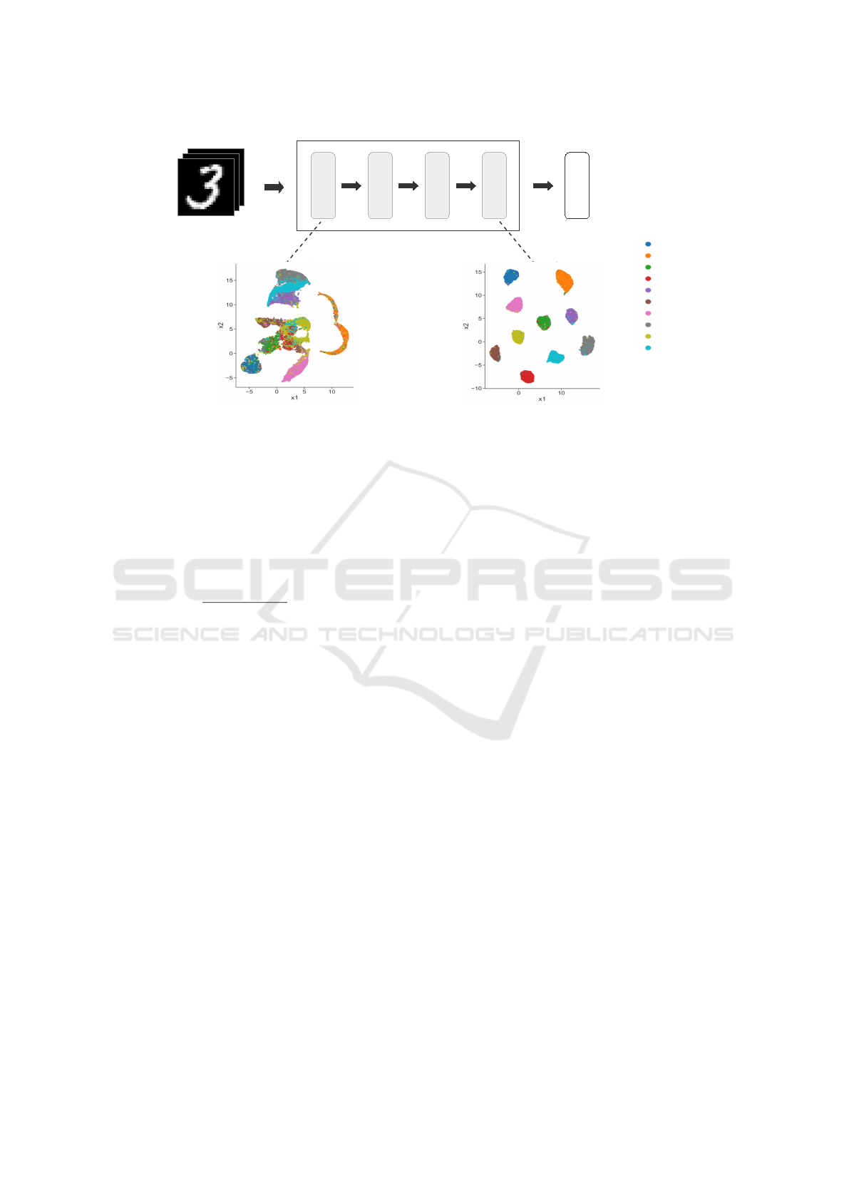
Figure 1: Visualization of the activations of the MNIST training samples at the ﬁrst layer (ConvLayer1) and the last layer

(FC-Layer) of the CNN model.

each cluster h

∈ 1,...,H

), we calculate the per-

cental class distribution statistic S

) of the training

samples in h

(i.e., for each class c: What percentage

is of class c?).

) =



c, p

(c)





c ∈ 1, ...,C



|(x

,y==c

|(x

(1)

However, to avoid outliers among the 1,...,C classes

in h

we only keep the classes c whose occurrence in

cluster h

is greater than a speciﬁed threshold t (e.g.,

distribution statistics S

) of all found clusters h

at layer l forms the class distribution statistic S

that layer. 3) For each layer l, the class distribution

statistic S

, the projection model r

, and the clustering

model g

are stored for the second stage of our method

at inference (section 3.2) according to the method in-

troduced by Lehmann and Ebner (2021).

In extension of the method from Lehmann and

Ebner (2021), we additionally calculate a layer score

for each layer l. We use these layer scores to com-

pute the credibility score in the second stage of our

method at inference (section 3.2). A layer score w

reﬂects the type of the calculated class distribution

statistic S

of the found clusters at that layer. As

pointed out by Zeiler and Fergus (2014), lower lay-

ers of a model detect low-level features (e.g., simple

shapes, edges), while higher layers of a model de-

tect high-level features (e.g., complex shapes, object

parts). Low-level features are typically shared among

different classes. An image of a class baseball player

and an image of a class soccer player, for instance,

share certain low-level features (e.g., simple shape

features of the body and face, the sportswear, or the

playing ﬁeld in the background). Thus, at lower lay-

ers, samples of different classes are typically close to

each other in feature space (as shown in Figure 1). As

a result, the class distribution statistics S

) at lower

layers tend to contain a large number of classes that

are rather uniformly distributed. This type of class

distribution is reﬂected in a low layer score. High-

level features, in contrast, are rather class-speciﬁc. As

a result, the class distribution statistics S

) tend to

contain a small number of classes that show a rather

imbalanced distribution. This is caused by the ob-

jective of model training to ﬁnd a linearly separable

representation of the different classes throughout the

layers of the model. Samples of the same class tend

to get closer to each other, while samples of differ-

ent classes tend to get farther apart from each other

(as shown in Figure 1). Thus, at the ﬁnal layer L,

each class distribution statistic S

) typically con-

tains a majority class with at least 90% occurrence in

the cluster h

. This type of class distribution is re-

ﬂected in a high layer score. To calculate the layer

scores we propose a simple method: 1) For each layer

l: (a) From all class distribution statistics S

) we

get the class with the highest and the class with the

second-highest occurrence. (b) We calculate the ab-

solute difference between the percentage of the high-

est and the second-highest class. As a result, we ob-

tain a score w

for each cluster h

. (c) To obtain the

layer score w

of layer l we take the average of these

cluster scores w

. 2) Finally, we normalize all layer

scores w

(i.e., their sum should be 1 ). As a result,

Calculating the Credibility of Test Samples at Inference by a Layer-wise Activation Cluster Analysis of Convolutional Neural Networks

we obtain the ﬁnal layer scores w

for each layer l.

After obtaining the class distribution statistic S

for each layer l from the training data, as suggested

by Lehmann and Ebner (2021), we additionally deter-

mine a cluster distribution statistic S

for each layer l

from a held-out test set. This test set has also been

sampled from the same distribution as the training

data, but the model f has not seen its samples (x

)

during training. Similar to Papernot and McDaniel

(2018), we use this test set to calibrate the credibility

score at inference (section 3.2). Therefore, we refer

to this test set as calibration set in the following. Cal-

culating the cluster distribution statistic S

for each

layer l from the calibration set requires the follow-

ing steps: 1) For each layer l: (a) We determine the

activation matrix A

in the same way as the activa-

tion matrix A

of the training data. (b) The projection

model r

and the clustering model g

are applied on

matrix A

. As a result, for each calibration sample x

we obtain the cluster h

into which x

falls. (c) For

each class c, we calculate the percental cluster distri-

bution statistic S

for each cluster h

: What percentage p

) of sam-

ples of class c is in cluster h

?).



, p

)





∈ 1,...,H



) =

|(x

,y==c

|(x

y==c

(2)

The set of cluster distribution statistics S

classes c at layer l forms the cluster distribution statis-

tic S

of that layer. 2) For each layer l, the cluster

distribution statistic S

is stored for the second stage

of our method at inference (section 3.2).

3.2 At Inference

At inference, we calculate the credibility score

credib(x

) ∈ [0, 1] of sample x

. For calculating the

credibility score we use the class distribution statis-

tic S

(from the training data), the cluster distribution

statistic S

(from the calibration data), the layer score

, the projection model r

, and the clustering model

of each layer l (all were obtained in the ﬁrst stage of

our method, as described in section 3.1). Calculating

the credibility score credib(x

) of sample x

requires

the following steps: 1) For each layer l: (a) We de-

termine the activation vector a

in the same way as

the activation vectors a

of the training samples (as

described in section 3.1). (b) The projection model r

and the clustering model g

are applied on vector a

As a result, we obtain the cluster h

into which x

falls. (c) From the class distribution statistic S

)

of cluster h

we get the set of classes cset

) that

are located in h

. 2) After obtaining the set of classes

cset

) from each layer l, we determine the inter-

section cset(x

) of cset

) over all layers 1, ..., L. If

cset(x

) is empty, we assume that sample x

is prob-

ably an OOD sample (as shown in Figure 2). This

follows from our assumption: An in-distribution sam-

ple of a certain class is close to other in-distribution

samples of the same class in feature space across all

layers of the model. In this case, cset(x

) must con-

tain one class at least. An OOD sample, in contrast,

is typically not close to in-distribution samples of the

same class across all layers. Thus, if cset(x

) is empty,

we return credib(x

) = 0. However, if cset(x

) is not

empty, we continue. 3) We assume that one of the

classes in cset(x

) may be the true class of x

. There-

fore, we calculate the credibility score credib(x

)

of x

for each class c

in cset(x

): (a) For each layer

l, we determine the probability of the class c

be-

ing located in cluster h

. To obtain a calibrated ver-

sion of this probability we use the cluster distribution

statistic S

) from the calibration set (the probabil-

ity can be obtained through S

)(h

)). We use the

probability to express the credibility. A high prob-

ability means that a sample of class c

is close to

a large number of calibration samples of the same

class in feature space of layer l. Thus, the sample is

probably an in-distribution sample (i.e., the credibil-

ity should be high). If any of the probabilities across

layer 1,..,L is 0, however, we assume sample x

probably an OOD sample. Again, this follows from

our assumption that an in-distribution sample of a cer-

tain class is close to other in-distribution samples of

the same class in feature space across all layers of the

model. Thus, if any of the probabilities among layers

1,...,L is 0, this assumption is violated, and we return

credib(x

) = 0. However, if all probabilities are non-

zero, we continue. (b) To obtain the total credibility

score credib(x

) for class c

, we take the average

of the probabilities S

)(h

). However, the proba-

bilities of the lower layers are typically low in general

because the clusters at lower layers contain a large

number of classes that are rather uniformly distributed

(as described in section 3.1). Thus, we put less em-

phasis on the lower layers by taking a weighted av-

erage of the probabilities S

)(h

) using the layer

scores w

as weights. 4) To obtain the total credibil-

ity score credib(x

) of the sample x

, we choose the

highest credibility score among all classes c

credib(x

) = max

credib(x

)

(3)

DeLTA 2022 - 3rd International Conference on Deep Learning Theory and Applications

max

classes = [red, blue]

credib(x

, red)

credib(x

, blue)

Softmax

Layer 1

Layer 2

Softmax

Layer 1

Layer 2

classes = Ø

credib(x

) = 0

is OOD!

credib(x

)

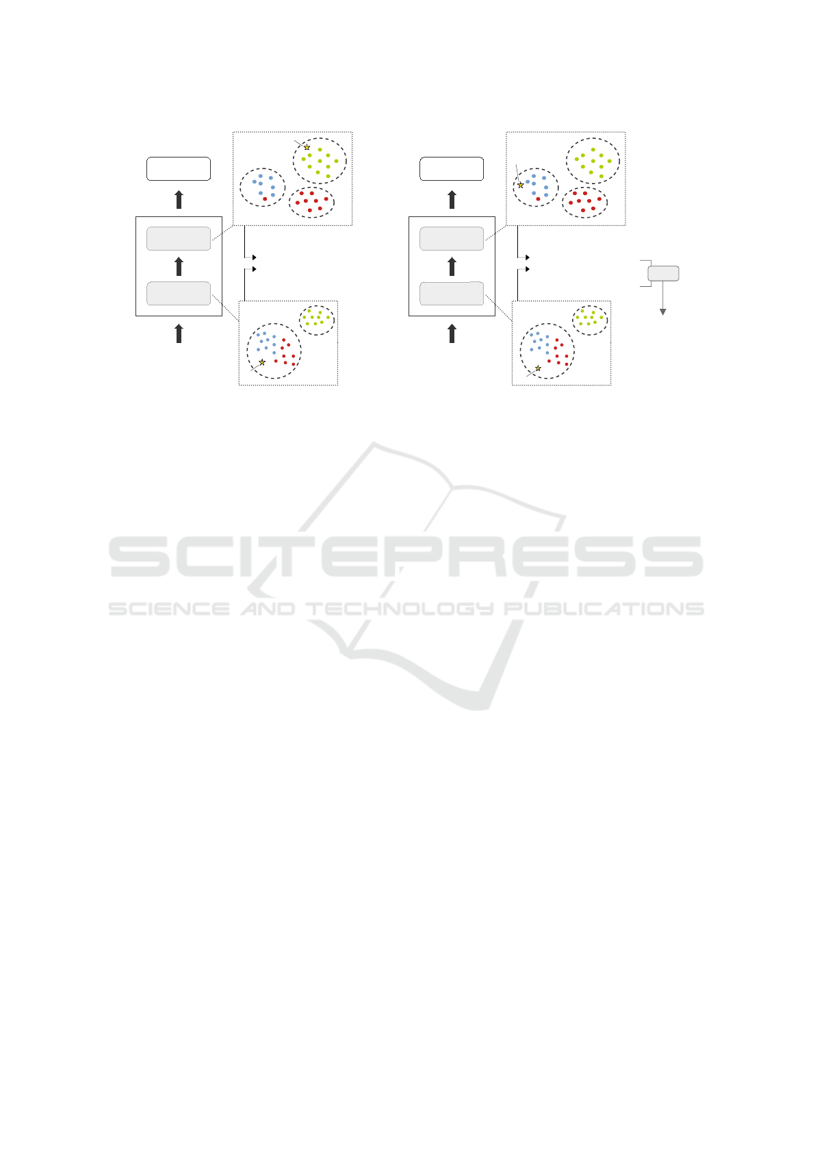
Figure 2: We check which classes are present in the cluster of the training samples into which the test sample falls at each

layer. If there is no common class across all layers, we assume it is an OOD sample (left). Otherwise, we calculate the test

sample credibility for each of the common classes, and use the maximum as the ﬁnal credibility of the test sample (right).

Our algorithm (in Python) for calculating the credibil-

ity score credib(x

) is shown below:

// get potential classes of x_i

cset = []

for l in range(0,L):

a = getActivations(x_i, l)

h = getCluster(r(l), g(l), a)

cset_l = getClasses(s_d(l, h))

cset = intersect(cset, cset_l)

// check if class set is empty

if cset is empty:

return 0 // x_i is OOD!

// get credbility score

credibList = []

for c in cset:

for l in range(0,L):

prob = getProb(s_t(l, c))

if prob == 0:

return 0 // x_i is OOD!

credibList.append(prob * w(l))

return max(credibList)

4 EXPERIMENTS

4.1 Experimental Setup

We conducted several experiments to test our method

in comparison to the DkNN method proposed by Pa-

pernot and McDaniel (2018). The objective of the

experiments was to compare the runtimes at infer-

ence and also the performance of both methods. The

experiments were conducted on the MNIST dataset

(60,000 training samples, 10,000 test samples) (Le-

Cun et al., 2010), the SVHN dataset (73,257 training

samples, 26,032 test samples) (Netzer et al., 2011),

and the CIFAR10 dataset (50,000 training samples,

10,000 test samples) (Krizhevsky, 2009). However,

before we could carry out any experiment, we ﬁrst

had to train a model on the respective training set

of each dataset. For MNIST and SVHN, we chose

the same CNN architecture for the model as Paper-

not and McDaniel (2018). The architecture for both

datasets consists of the following layers: ConvLayer1

(ﬁlters: 64, kernel size: 8, stride: 2) - ConvLayer2

(ﬁlters: 128, kernel size: 6, stride: 2) - ConvLayer3

(ﬁlters: 128, kernel size: 5) - fully-connected out-

put layer (size: 10). Each ConvLayer uses ReLU as

activation function. To train the model on MNIST,

we used the following training parameters: 6 training

epochs, Adam optimizer, learning rate (LR) of 0.001,

kaiming uniform weight initialization. Our MNIST

model achieves a performance of 99.04% accuracy

on the MNIST test dataset. To train the model on

SVHN, we used the following training parameters: 18

training epochs, Adam optimizer, base LR of 0.001,

multi-step LR-schedule (step at epoch: (10,14,16),

gamma: 0.1), kaiming uniform weight initialization.

Our SVHN model achieves a performance of 89.95%

accuracy on the SVHN test dataset. For CIFAR10,

which was not used for the experiments conducted by

Papernot and McDaniel (2018), we chose a 20-layer

ResNet architecture for the model as used by Zhang

et al. (2019). To train the model on CIFAR10, we

used the following training parameters: data augmen-

tation (mixup, random horizontal ﬂip, random crop),

200 training epochs, SGD optimizer, base LR of 0.1,

cosine-annealing LR-schedule, ﬁxup weight initial-

Calculating the Credibility of Test Samples at Inference by a Layer-wise Activation Cluster Analysis of Convolutional Neural Networks

ization (Zhang et al., 2019). Our CIFAR10 model

achieves a performance of 92.47% accuracy on the

CIFAR10 test dataset.

After training a model for each dataset, we fed

an in-distribution test set as well as different types of

OOD test sets to each model and calculated the cred-

ibility for the samples of each test set. The credibil-

ity score should be high for in-distribution samples

and low for OOD samples. For both, our method and

the DkNN method, we used a calibration set size of

750 samples. This size was also used by Papernot and

McDaniel (2018) in their experiments. The calibra-

tion samples were randomly selected from the test set

of each dataset. As in-distribution test set, we used

the test set of each dataset excluding the samples that

were used for the calibration set. As OOD test set,

we used a natural OOD test set (section 4.2) as well

as different types of adversarial test sets (section 4.3).

The adversarial test sets were created from the test set

of each dataset excluding the samples used for the cal-

ibration set. For MNIST and SVHN, we used the ac-

tivations of all layers to calculate the credibility score

using our method as well as the DkNN method (Con-

vLayers: activations after ReLU). For CIFAR10, we

selected the following layer activations to calculate

the credibility score using our method as well as the

DkNN method: the ﬁrst ConvLayer activations (af-

ter ReLU), the output activations from the 3 ResNet

blocks, the Global-Average-Pooling layer activations,

and the fully-connected output layer activations. Ad-

ditionally, we needed to select a value for the param-

eter t of our method. We chose the following values

for t: 0.01, 0.05, and 0.1. Finally, in each experiment,

we calculated the mean credibility of the samples of

the test set and measured the calculation runtime at

inference.

4.2 Natural OOD Samples

We evaluated the performance of our method in com-

parison to the DkNN method on natural OOD sam-

ples. In section 4.1, we trained a model for the

MNIST, SVHN, and CIFAR10 dataset. To test the

performance of both, our method and the DkNN

method, we fed a respective natural OOD test set into

each of these models. Each OOD test set contains

samples that have not been drawn from the same dis-

tribution as the samples used for training the model.

We used the following natural OOD test sets: the

KMNIST test dataset (Clanuwat et al., 2018) for the

model trained on MNIST (10,000 test samples, test

performance: 7.59% accuracy), the CIFAR10 test

dataset for the model trained on SVHN (10,000 test

samples, test performance: 9.24% accuracy), and the

SVHN test dataset for the model trained on CIFAR10

(26,032 test samples, test performance: 9.35% ac-

curacy). For each OOD test set, we calculated the

mean credibility score of all test samples using (a) our

method and (b) the DkNN method. The results of our

tests are shown in Table 1.

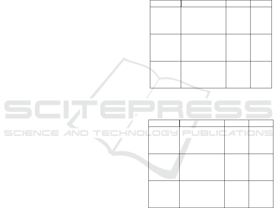
Table 1: Mean credibility scores of our method compared

to DkNN for in-distribution samples (Testset) and natural

OOD samples (OOD). For in-distribution samples a higher

score is better, while for OOD samples a lower score is bet-

ter.

Dataset Method Testset OOD

MNIST DkNN 0.799 0.081

Ours (t = 0.01) 0.889 0.164

Ours (t = 0.05) 0.882 0.124

Ours (t = 0.1) 0.880 0.124

SVHN DkNN 0.501 0.146

Ours (t = 0.01) 0.702 0.427

Ours (t = 0.05) 0.635 0.233

Ours (t = 0.1) 0.451 0.145

CIFAR10 DkNN 0.526 0.221

Ours (t = 0.01) 0.844 0.565

Ours (t = 0.05) 0.749 0.452

Ours (t = 0.1) 0.353 0.150

Table 2: Runtimes at inference of our method compared to

DkNN (in seconds) for in-distribution samples (Testset) and

natural OOD samples (OOD). A lower runtime is better.

Dataset Method Testset OOD

MNIST DkNN 304.4 242.3

Ours (t = 0.01) 24.1 28.3

Ours (t = 0.05) 24.4 28.6

Ours (t = 0.1) 23.3 28.9

SVHN DkNN 1137.7 315.0

Ours (t = 0.01) 79.1 39.6

Ours (t = 0.05) 83.4 39.7

Ours (t = 0.1) 77.5 42.9

CIFAR10 DkNN 680.8 1850.3

Ours (t = 0.01) 155.5 400.8

Ours (t = 0.05) 143.0 405.9

Ours (t = 0.1) 152.5 400.1

As shown in Table 1, for t = 0.01 and t = 0.05, we

obtain a higher credibility score on the in-distribution

samples compared to DkNN. However, the DkNN

method achieves a lower credibility score on the OOD

samples. Increasing parameter t to t = 0.1 improves

our method on OOD samples. We even achieve a

slightly lower credibility score than DkNN on the

OOD test set for the SVHN and CIFAR10 model.

However, the credibility score for the in-distribution

samples is lower compared to DkNN in this case.

Nevertheless, the main objective of our experiments

was to examine whether our method is faster than the

DkNN method at inference. Therefore, we also mea-

DeLTA 2022 - 3rd International Conference on Deep Learning Theory and Applications

Table 3: Mean credibility scores of our method compared to DkNN for in-distribution samples (Testset) and adversarial

samples (FGSM, BIM, PGD, PGD

DLR

). For in-distribution samples a higher score is better, while for OOD samples a lower

score is better.

Dataset Method Testset FGSM BIM PGD PGD

DLR

MNIST DkNN 0.799 0.136 0.085 0.087 0.070

Ours (t = 0.01) 0.889 0.237 0.207 0.152 0.178

Ours (t = 0.05) 0.882 0.179 0.165 0.124 0.154

Ours (t = 0.1) 0.880 0.173 0.166 0.122 0.152

SVHN DkNN 0.501 0.237 0.309 0.296 0.215

Ours (t = 0.01) 0.702 0.571 0.655 0.636 0.563

Ours (t = 0.05) 0.635 0.387 0.500 0.473 0.362

Ours (t = 0.1) 0.451 0.226 0.289 0.273 0.198

CIFAR-10 DkNN 0.526 0.176 0.180 0.220 0.285

Ours (t = 0.01) 0.844 0.314 0.523 0.573 0.651

Ours (t = 0.05) 0.749 0.177 0.442 0.461 0.539

Ours (t = 0.1) 0.353 0.043 0.025 0.031 0.152

Table 4: Runtimes at inference of our method compared to DkNN (in seconds) for in-distribution samples (Testset) and

adversarial samples (FGSM, BIM, PGD, PGD

DLR

). A lower runtime is better.

Dataset Method Testset FGSM BIM PGD PGD

DLR

MNIST DkNN 304.4 273.8 286.8 287.3 281.6

Ours (t = 0.01) 24.1 26.6 27.5 28.1 31.2

Ours (t = 0.05) 24.4 26.0 28.6 28.8 28.1

Ours (t = 0.1) 23.3 27.5 28.3 28.5 29.2

SVHN DkNN 1137.7 1054.8 1195.0 1230.7 1288.2

Ours (t = 0.01) 79.1 83.2 85.9 77.8 87.5

Ours (t = 0.05) 83.4 85.7 82.0 90.2 90.4

Ours (t = 0.1) 77.5 88.6 92.4 90.4 88.9

CIFAR-10 DkNN 680.8 738.9 784.6 796.1 736.4

Ours (t = 0.01) 155.5 177.2 166.1 170.3 166.5

Ours (t = 0.05) 143.0 162.4 164.3 164.1 155.4

Ours (t = 0.1) 152.5 177.5 164.9 169.3 165.4

sured the runtimes at inference of both, our method

and the DkNN method, for each OOD test set. The

result are shown in Table 2. As shown in the table, our

method is signiﬁcantly faster than the DkNN method.

4.3 Adversarial Samples

Similar to our experiments for natural OOD samples

in section 4.2, we also evaluated the performance

of our method in comparison to the DkNN method

on adversarial samples. We created the adversarial

test sets from the respective in-distribution test set of

each dataset (MNIST, SVHN, CIFAR10) using the

Python library torchattacks (Kim, 2020). To create

the adversarial samples from the MNIST test dataset,

we used the following methods: FGSM (Goodfellow

et al., 2015) (ε = 0.25, test performance: 8.05% accu-

racy), BIM (Kurakin et al., 2017) (ε = 0.25, α = 0.01,

i = 100, test performance: 0.04% accuracy), PGD

(Madry et al., 2018) (ε = 0.2, α = 2/255, i = 40, test

performance: 2.46% accuracy), and PGD

DLR

(Croce

and Hein, 2020) (ε = 0.3, α = 2/255, i = 40, test per-

formance: 0.85% accuracy). To create the adversarial

samples from the SVHN test dataset, we used the fol-

lowing methods: FGSM (ε = 0.05, test performance:

2.72% accuracy), BIM (ε = 0.05, α = 0.005, i = 20,

test performance: 0.79% accuracy), PGD (ε = 0.04,

α = 2/255, i = 40, test performance: 2.42% accu-

racy), and PGD

DLR

(ε = 0.3, α = 2/255, i = 40,

test performance: 3.48% accuracy). To create the

adversarial samples from the CIFAR10 test dataset,

we used the following methods: FGSM (ε = 0.1,

test performance: 13.21% accuracy), BIM (ε = 0.1,

α = 0.05, i = 20, test performance: 0.84% accuracy),

PGD (ε = 0.3, α = 2/255, i = 40, test performance:

0.93% accuracy), and PGD

DLR

(ε = 0.3, α = 2/255,

i = 40, test performance 28.0% accuracy). We fed the

test samples of each adversarial test set into the re-

spective model. Then, we calculated the mean cred-

ibility score of all test samples using (a) our method

and (b) the DkNN method. The results of our tests

are shown in Table 3. As shown in the table, we ob-

Calculating the Credibility of Test Samples at Inference by a Layer-wise Activation Cluster Analysis of Convolutional Neural Networks

tain similar results as from our experiments in sec-

tion 4.2. A higher credibility score is obtained on in-

distribution samples compared to DkNN for t = 0.01

and t = 0.05. However, the score on adversarial OOD

samples is also higher. Again, increasing parame-

ter t to t = 0.1 improves our method on adversarial

OOD samples. We even slightly outperform DkNN

on the adversarial test sets for the SVHN and CI-

FAR10 model. However, as in section 4.2, the cred-

ibility score for the in-distribution samples is lower

compared to DkNN in this case. Nevertheless, the

main objective of our experiments was to examine

whether our method is faster than the DkNN method

at inference. Therefore, we also measured the run-

times at inference of both, our method and the DkNN

method, for each adversarial OOD test set. The re-

sults are shown in Table 4. As shown in the table, our

method is signiﬁcantly faster than the DkNN method.

5 CONCLUSION

In section 1, we stated the two goals of our research

study. Our ﬁrst goal was to examine if information

from clusters of the layer activations of a model can

be used to compute the credibility of a test sample at

inference (regarding that model). In section 4, our

experiments show that this cluster information can

be used for the credibility calculation. Our method

computes meaningful credibility scores. The calcu-

lated credibility scores are signiﬁcantly higher for in-

distribution samples than for OOD samples. Our sec-

ond goal was to perform a comprehensive comparison

of our method with the DkNN method in terms of run-

time at inference. We performed the comparison on a

natural OOD test set (section 4.2) and several adver-

sarial test sets (section 4.3) for the MNIST, SVHN

and CIFAR10 dataset. The results of our comparison

show that our method is signiﬁcantly faster than the

DkNN method. This is an important result. A method

for detecting OOD samples must be fast at inference

in order to be practical. Moreover, our method almost

achieves the performance of DkNN. The parameter t

of our method is crucial. For t = 0.01 and t = 0.05,

our method performs worse than the DkNN method

on OOD samples but better on in-distribution sam-

ples. Increasing t to t = 0.1 improves the performance

of our method on OOD samples. We achieve a similar

or sometimes even slightly better performance than

DkNN for t = 0.1. However, the performance of our

method on in-distribution samples of SVHN and CI-

FAR10 decreases in this case. In future work, we aim

to further improve the performance of our method.

REFERENCES

Andoni, A. and Indyk, P. (2006). Near-optimal hashing al-

gorithms for approximate nearest neighbor in high di-

mensions. In Foundations of Computer Science, 2006.

FOCS’06. 47th Annual IEEE Symposium on, pages

459–468. IEEE.

Biggio, B., Corona, I., Maiorca, D., Nelson, B.,

Srndi

c, N.,

Laskov, P., Giacinto, G., and Roli, F. (2013). Evasion

attacks against machine learning at test time. In Bloc-

keel, H., Kersting, K., Nijssen, S., and

Zelezn

y, F.,

editors, ECML PKDD, pages 387–402, Berlin - Hei-

delberg, Germany. Springer.

Carrara, F., Falchi, F., Caldelli, R., Amato, G., and Be-

carelli, R. (2019). Adversarial image detection in deep

neural networks. Multimedia Tools and Applications,

78(3):2815–2835.

Chen, B., Carvalho, W., Baracaldo, N., Ludwig, H., Ed-

wards, B., Lee, T., Molloy, I., and Srivastava, B.

(2019a). Detecting backdoor attacks on deep neu-

ral networks by activation clustering. In Espinoza,

H.,

O h

Eigeartaigh, S., Huang, X., Hern

andez-Orallo,

J., and Castillo-Effen, M., editors, Workshop on

SafeAI@AAAI, volume 2301 of CEUR Workshop,

Honolulu, HI, USA. ceur-ws.org.

Chen, T., Navratil, J., Iyengar, V., and Shanmugam, K.

(2019b). Conﬁdence scoring using whitebox meta-

models with linear classiﬁer probes. In Chaudhuri,

K. and Sugiyama, M., editors, AISTATS, volume 89,

pages 1467–1475, Naha, Japan. PMLR.

Clanuwat, T., Bober-Irizar, M., Kitamoto, A., Lamb, A.,

Yamamoto, K., and Ha, D. (2018). Deep learning for

classical japanese literature. ArXiv, abs/1812.01718.

Cohen, G., Sapiro, G., and Giryes, R. (2020). Detecting ad-

versarial samples using inﬂuence functions and near-

est neighbors. In CVPR, pages 14441–14450, Seattle,

WA, USA. IEEE.

Croce, F. and Hein, M. (2020). Reliable evaluation of

adversarial robustness with an ensemble of diverse

parameter-free attacks. In ICML, volume 119, pages

2206–2216. PMLR.

Gal, Y. (2016). Uncertainty in Deep Learning. PhD thesis,

Univ of Cambridge.

Gal, Y. and Ghahramani, Z. (2016). Dropout as a bayesian

approximation: Representing model uncertainty in

deep learning. In Balcan, M. and Weinberger, K., edi-

tors, ICML, volume 48, pages 1050–1059, New York,

NY, USA. PMLR.

Goodfellow, I., Shlens, J., and Szegedy, C. (2015). Ex-

plaining and harnessing adversarial examples. In Ben-

gio, Y. and LeCun, Y., editors, ICLR, San Diego, CA,

USA.

Grosse, K., Manoharan, P., Papernot, N., Backes, M., and

McDaniel, P. (2017). On the (statistical) detection of

adversarial examples. ArXiv, abs/1702.06280.

He, K., Zhang, X., Ren, S., and Sun, J. (2016). Deep resid-

ual learning for image recognition. In CVPR, pages

770–778, Las Vegas, NV, USA. IEEE.

Hendrycks, D. and Gimpel, K. (2017). A baseline for de-

DeLTA 2022 - 3rd International Conference on Deep Learning Theory and Applications

tecting misclassiﬁed and out-of-distribution examples

in neural networks. In ICLR, Toulon, France.

Hendrycks, D., Mazeika, M., Kadavath, S., and Song,

D. (2019). Using self-supervised learning can im-

prove model robustness and uncertainty. In Wallach,

H., Larochelle, H., Beygelzimer, A., d'Alch

e-Buc, F.,

Fox, E., and Garnett, R., editors, NeurIPS, volume 32,

pages 15637–15648, Vancouver, CA. CAI.

Hendrycks, D., Zhao, K., Basart, S., Steinhardt, J., and

Song, D. (2020). Natural adversarial examples. ArXiv,

abs/1907.07174.

Huang, H., Li, Z., Wang, L., Chen, S., Dong, B., and

Zhou, X. (2021). Feature space singularity for out-

of-distribution detection. In Espinoza, H., McDer-

mid, J., Huang, X., Castillo-Effen, M., Chen, X. C.,

Hern

andez-Orallo, J.,

O h

Eigeartaigh, S., and Mallah,

R., editors, Workshop on SafeAI@AAAI, volume 2808

of CEUR Workshop. ceur-ws.org.

Kim, H. (2020). Torchattacks: A pytorch repository for

adversarial attacks. ArXiv, abs/2010.01950.

Krizhevsky, A. (2009). Learning multiple layers of features

from tiny images. Technical report, Univ of Toronto.

Krizhevsky, A., Sutskever, I., and Hinton, G. E. (2012).

Imagenet classiﬁcation with deep convolutional neu-

ral networks. In Pereira, F., Burges, C. J. C., Bottou,

L., and Weinberger, K. Q., editors, NIPS, volume 25,

pages 1097–1105, Lake Tahoe, NV, USA. CAI.

Kurakin, A., Goodfellow, I. J., and Bengio, S. (2017). Ad-

versarial examples in the physical world. In ICLR,

Toulon, France.

LeCun, Y., Cortes, C., and Burges, C. (2010). Mnist

handwritten digit database. ATT Labs [Online],

http://yann.lecun.com/exdb/mnist, 2.

Lee, K., Lee, H., Lee, K., and Shin, J. (2018a). Training

conﬁdence-calibrated classiﬁers for detecting out-of-

distribution samples. In ICLR, Vancouver, CA.

Lee, K., Lee, K., Lee, H., and Shin, J. (2018b). A simple

uniﬁed framework for detecting out-of-distribution

samples and adversarial attacks. In Bengio, S., Wal-

lach, H., Larochelle, H., Grauman, K., Cesa-Bianchi,

N., and Garnett, R., editors, NeurIPS, volume 31, page

7167–7177, Montreal, CA. CAI.

Lehmann, D. and Ebner, M. (2021). Layer-wise activation

cluster analysis of cnns to detect out-of-distribution

samples. In Farkas, I., Masulli, P., Otte, S., and

Wermter, S., editors, Proc of the 30th Int Conf on Ar-

tiﬁcial Neural Networks ICANN 2021, Lecture Notes

in CS, pages 214–226, Berlin, Germany. Springer.

Li, X. and Li, F. (2017). Adversarial examples detection in

deep networks with convolutional ﬁlter statistics. In

ICCV, pages 5775–5783, Venice, Italy. IEEE.

Liang, S., Li, Y., and Srikant, R. (2018). Enhancing the reli-

ability of out-of-distribution image detection in neural

networks. In ICLR, Vancouver, CA.

Lin, Z., Roy, S. D., and Li, Y. (2021). Mood: Multi-level

out-of-distribution detection. In CVPR, pages 15308–

15318. IEEE.

Ma, X., Li, B., Wang, Y., Erfani, S. M., Wijewickrema, S.,

Schoenebeck, G., Houle, M. E., Song, D., and Bailey,

J. (2018). Characterizing adversarial subspaces using

local intrinsic dimensionality. In ICLR, Vancouver,

CA.

Machado, G. R., Silva, E., and Goldschmidt, R. R. (2021).

Adversarial machine learning in image classiﬁcation:

A survey toward the defender’s perspective. ACM

Comput. Surv., 55(1):1–38.

MacQueen, J. B. (1967). Some methods for classiﬁcation

and analysis of multivariate observations. In Cam,

L. M. L. and Neyman, J., editors, Berkeley Symp on

Math Stat and Prob, volume 1, pages 281–297. Univ

of Calif Press.

Madry, A., Makelov, A., Schmidt, L., Tsipras, D., and

Vladu, A. (2018). Towards deep learning models re-

sistant to adversarial attacks. In ICLR, Vancouver, CA.

McInnes, L., Healy, J., and Melville, J. (2018). UMAP:

Uniform manifold approximation and projection for

dimension reduction. ArXiv, abs/1802.03426.

Meng, D. and Chen, H. (2017). Magnet: A two-pronged de-

fense against adversarial examples. In SIGSAC, page

135–147, Dallas, TX, USA. ACM.

Metzen, J. H., Genewein, T., Fischer, V., and Bischoff, B.

(2017). On detecting adversarial perturbations. In

ICLR, Toulon, France.

Netzer, Y., Wang, T., Coates, A., Bissacco, A., Wu, B., and

Ng, A. Y. (2011). Reading digits in natural images

with unsupervised feature learning. In NIPS Workshop

on Deep Learning and Unsupervised Feature Learn-

ing.

Papernot, N. and McDaniel, P. (2018). Deep k-nearest

neighbors: Towards conﬁdent, interpretable and ro-

bust deep learning. ArXiv, abs/1803.04765.

Pearson, K. (1901). LIII. On lines and planes of closest

ﬁt to systems of points in space. London, Edinburgh

Dublin Philos Mag J Sci, 2(11):559–572.

Sastry, C. S. and Oore, S. (2020). Detecting out-of-

distribution examples with gram matrices. In ICML,

volume 119, pages 8491–8501. PMLR.

Szegedy, C., Zaremba, W., Sutskever, I., Bruna, J., Erhan,

D., Goodfellow, I. J., and Fergus, R. (2014). Intrigu-

ing properties of neural networks. In Bengio, Y. and

LeCun, Y., editors, ICLR, Banff, CA.

Zeiler, M. D. and Fergus, R. (2014). Visualizing and un-

derstanding convolutional networks. In Fleet, D., Pa-

jdla, T., Schiele, B., and Tuytelaars, T., editors, ECCV,

number PART 1 in Lecture Notes in CS, pages 818–

833, Zurich, CH. Springer.

Zhang, H., Dauphin, Y. N., and Ma, T. (2019). Fixup ini-

tialization: Residual learning without normalization.

ArXiv, abs/1901.09321.

Calculating the Credibility of Test Samples at Inference by a Layer-wise Activation Cluster Analysis of Convolutional Neural Networks