Reduced CP Representation of Multilinear Models

Niklas J

ores

1 a

, Christoph Kaufmann

1,2,4 b

, Leona Schnelle

2 c

, Carlos Cateriano Y

nez

1,2,3 d

Georg Pangalos

1 e

and Gerwald Lichtenberg

2 f

Application Center for Integration of Local Energy Systems, Fraunhofer IWES, Hamburg, Germany

Faculty of Life Science, HAW Hamburg, Germany

Universitat Polit

ecnica de Val

encia, Instituto Universitario de Autom

atica e Inform

atica Industrial, Val

encia, Spain

Centre d’Innovaci

o Tecnol

ogica en Convertidors Est

atics i Accionaments (CITCEA),

Departament d’Enginyeria El

ectrica, Universitat Polit

ecnica de Catalunya (UPC), Barcelona, Spain

Keywords:

Multilinear Systems, Tensor Decomposition.

Abstract:

Large and highly complex systems can be found in various application areas. Modeling these systems requires

appropriate representation of the underlying phenomena. Furthermore, due to the large dimensions efﬁcient

simulation and low memory requirements are needed for such models. Multilinear modeling is a promising

approach to address these challenges. In this paper, we introduce a reduced canonical polyadic (CP) repre-

sentation for implicit time-invariant multilinear (iMTI) models. This representation is capable of storing large

models with very low memory requirements. This is particularly useful for efﬁcient analyses of large systems

with numerous inputs and states.

1 INTRODUCTION

Modeling and simulation of complex systems is an

active ﬁeld of research. Currently, e.g., in the ﬁeld

of modeling energy systems co-simulation method-

ology is used as one approach to address the high

complexity, while maintaining a realistic representa-

tion (L

opez et al., 2019; Farrokhseresht et al., 2021;

Wiens et al., 2021; Vogt et al., 2018). However, mod-

eling of such large and complex systems while cap-

turing the relevant dynamics results in large computa-

tional resources and simulation times with the exist-

ing modeling approaches. Therefore, more computa-

tional power, more efﬁcient algorithms and new mod-

eling strategies are required (F. Milano et al., 2018).

Focusing on modeling strategies, a possibility is

to rethink the fundamental question: Which class of

models has the potential to cover all relevant non-

linear dynamics and at the same time enables efﬁ-

https://orcid.org/0000-0003-2471-3892

https://orcid.org/0000-0002-0666-1104

https://orcid.org/0000-0002-2600-8110

https://orcid.org/0000-0001-5261-2568

https://orcid.org/0000-0001-5094-8033

https://orcid.org/0000-0001-6032-0733

cient simulations as well as analysis and design al-

gorithms? For some large scale complex application

domains with similar modeling problems, recent re-

search shows that multilinearity and tensor decom-

position methods could lead to breakthroughs (Ver-

straete et al., 2008).

In recent years the multilinear modeling frame-

work have been introduced ﬁrst in an explicit form

by (Pangalos et al., 2013) and then in the more gen-

eral implicit form (Lichtenberg et al., 2022). The ad-

vantage of multilinear models is, that some nonlinear

phenomena can be modeled while still maintaining

an efﬁcient and structured representation. Applica-

tion examples range from heating systems (Pangalos

et al., 2013) over chemical reactions (Kruppa et al.,

2014) to energy systems (Lichtenberg et al., 2022). In

addition, efﬁcient simulation is possible, when using

decompositions. However, the multilinear model is

still an approximation and therefore, not as exact as

the nonlinear model. In addition, the tools for mul-

tilinear modeling are not yet standard and further de-

velopment is required.

Regarding controller synthesis, approaches to deal

with multilinear models in the application domain

of heating systems are given in (Pangalos, 2016;

Kruppa, 2018). The heating sector has the advantage

252

Jöres, N., Kaufmann, C., Schnelle, L., Yáñez, C., Pangalos, G. and Lichtenberg, G.

Reduced CP Representation of Multilinear Models.

DOI: 10.5220/0011273100003274

In Proceedings of the 12th International Conference on Simulation and Modeling Methodologies, Technologies and Applications (SIMULTECH 2022), pages 252-259

ISBN: 978-989-758-578-4; ISSN: 2184-2841

of relatively slow processes, which corresponds to

large time constants. This is in contrast to the electri-

cal energy system, where the need to efﬁcient simula-

tion is therefore even bigger. In this contribution, we

focus on improving the performance and memory re-

quirements of multilinear time-invariant (MTI) mod-

els - as a prerequisite to meet real-time constraints for

enabling model-based control of large scale systems.

First an introduction into multilinear functions is

given. This is followed by the explanation of explicit

multilinear time-invariant (eMTI) models, which in-

cludes decomposition, normalization and lineariza-

tion of eMTI models. The extension of eMTI is then

given with implicit multilinear time-invariant (iMTI)

models. The last chapter shows how an iMTI model

can be represented with very low memory require-

ments. A conclusion and further research is stated in

the end.

2 MULTILINEAR FUNCTIONS

In this section different formats for multilinear func-

tions are discussed as basis for the following model-

ing concepts. A multilinear function can be described

by the factored polynomial

f (x)=

∑

k=1

∏

i=1

( f

i,k

+ f

i,k

), (1)

with a total number of 2rn parameters, where f

i,k

∈ R

and f

i,k

∈ R\{0} for all i = 1,2...n and k = 1,2...r,

and x

are the variables of the function and k describes

the number of the addend.

Remark: The example

(4 + 2x

)(3 + x

) = (2 + x

)(6 + 2x

shows, that the representation (1) is not unique.

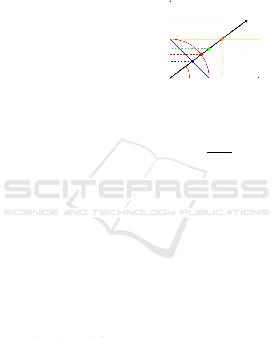
Each factor of the polynomial (1) can be visual-

ized in a 2-D Cartesian coordinate system, where the

two parameters f

and f

create a vector with one

component in direction of the 1-axis and one compo-

nent in direction of the x

-axis as shown in Figure 1

with an example vector ( f

)

Next, we will use normalization to get unique rep-

resentations, as the following example does for differ-

ent norms,



1 +



(2 + x) = 2





If we normalize this vector with the euclidean 2-

norm condition to the length of one, the new vector

points to the intersection S

of the original vector and

the unit circle in Figure 1. The intercepts of the 2-

norm normalized vector are then given by sinα and

0 1

sinα

Figure 1: Normalized factor representation.

cosα and the 2-norm normalized polynomial

f (x)=

∑

k=1

α,k

∏

i=1

(cosα

i,k

+ sinα

i,k

)

, (2)

has with

i,k

=atan2



i,k

, f

1i,k



, (3)

α,k

∏

i=1

1i,k

+ f

i,k

, (4)

a much smaller number r(n + 1) of parameters as (1).

The atan2 describes the four-quadrant inverse tangent

which gives the angle between the ﬁrst and the second

argument in radians.

Similarly, the polynomial can be transformed in a

1-norm representation as shown by the intersection S

with the blue line as

f (x)=

∑

k=1

h,k

∏

i=1

(1 − h

i,k

+ h

i,k

)

, (5)

where the new parameters are

i,k

+ f

i,k

and λ

h,k

∏

i=1



i,k

+ f

i,k



.(6)

By ﬁxing the x-axis coordinate to one, the inter-

section S

lead to a polynomial

f (x)=

∑

k=1

z,k

∏

i=1

i,k

+ x

)

, (7)

with the parameters

i,k

1i,k

i,k

and λ

z,k

∏

i=1

i,k

, (8)

and the zeros x

i,k

= −z

i,k

of each factor of the polyno-

mial.

The last intersection point S

with the green line

in Figure 1 ﬁxes the 1-axis coordinate to one, leading

to a representation

f (x)=

∑

k=1

∏

i=1

(1 + p

i,k

)

, (9)

Reduced CP Representation of Multilinear Models

253

called ‘sparse’ in the following and having the param-

eters

i,k

and λ

∏

i=1

i,k

j,k

, (10)

for all f

j,k

6= 0. In case of f

j,k

= 0, the factor vector

is pointing on the x

-axis and the parameter p

j,k

→ ∞.

Like in time-constant formulation of transfer func-

tions, the polynomial can then be represented by

f (x) =

∑

k=1

∏

(1 + p

i,k

) , (11)

and the factors λ

∏

i,k

∏

j,k

adjusted.

The sparse representation offers advantages for

modeling large systems and is mainly used in the next

sections in this paper, which are outlined by Figure 2

and linked to the related examples and equations in

the sequel.

eMTI

(12)

Full

CP tensor

(14)

1. Multilinear model classes 2. Tensor representation

4. Linearization

Reduced

CP tensor

(18)

3. Normalization

5. Formating

iMTI

(36)

Decomposition

Linear

(26)

Minimal

(4)

Linearization Encoding

Decoding

1-norm

(23)

2-norm

(22)

Zero

(24)

Sparse

(25)

Figure 2: Multilinear modeling steps.

3 EXPLICIT MULTILINEAR

MODELS

An eMTI state-space model in continuous time can

be expressed by using the contracted tensor prod-

uct, (Pangalos, 2016)

x =

M(x,u)

, (12)

with the parameter tensor F ∈ R

n+m

z }| {

2 × ... × 2×n

, where n

declares the number of states, and m is the number

of inputs. For brevity, we consider no extra output

equations, but the general approach could be easily

extended to this case if needed (Pangalos, 2016). The

next example will be a running one throughout this

paper.

Example 3.1. Consider a second-order eMTI model

with two states x

and one input u



˙x





0.4u + 0.2x

+ 0.08ux

+ 0.06x

0.6 + 0.24x

+ 0.94x

+ 0.296x



(13)

The full parameter tensor F ∈ R

2×2×2×2

has the fol-

lowing nonzero elements

F(1,1, 2,1) = 0.4,

F(1,2, 1,1) = 0.2,

F(2,1, 2,1) = 0.08,

F(2,2, 1,1) = 0.06,

F(1,1, 1,2) = 0.6,

F(2,1, 1,2) = 0.24,

F(1,2, 1,2) = 0.94,

F(2,2, 1,2) = 0.296,

(14)

where the indices are ordered from x

, x

over u to φ,

which speciﬁes the corresponding row in (13).

3.1 Decomposition

Because of the similarity with the factorization dis-

cussed in Section 2, we focus on canonical polyadic

(CP)-decompostions of the parameter tensor F as one

of the methods, e.g., given in (Kolda and Bader,

2009). The decomposed tensor of rank r is given

by factor matrices F

∈ R

2×r

for all states and inputs

with the common index i = 1,.. .n + m together with

the matrix F

∈ R

n×r

distributing factors over state

derivatives and jointly represented by

F =



,.. .,F



. (15a)

As the monomial tensor has a rank-1 decomposition

M(x,u) =





,···,









,···,





(15b)

the model (12) can also be represented by the CP-

factors, (Pangalos, 2016),

x = F







~ ··· ~









~ ··· ~





, (16)

where ~ stands for the Hadamard (element-wise)

product. Any internal structure of the model can be

exploited to ﬁnd a more compact CP representation

as the full tensor, which is motivated by the running

example next.

SIMULTECH 2022 - 12th International Conference on Simulation and Modeling Methodologies, Technologies and Applications

254

Example 3.2. The full representation can be rewrit-

ten as CP model of rank 8 directly from the 8 addends

in (13). Due to the duplication of variable combina-

tions x

and x

, the model can be reduced to rank 6

with factor matrices



1 1 0 0 1 0

0 0 1 1 0 1



, (17a)



1 0 1 0 1 1

0 1 0 1 0 0



, (17b)



0 1 0 1 1 1

1 0 1 0 0 0



, (17c)



0.4 0.2 0.08 0.06 0 0

0 0.94 0 0.296 0.6 0.24



. (17d)

The question of whether the parameter tensor F

could be further reduced, i.e. represented by a lower

number of factors is related to the non-trivial problem

of tensor rank determination (Kolda and Bader, 2009).

For the running example, the answer is yes.

Example 3.3. The tensor F of the running example is

representable as rank 4 shown by the factor matrices



0.4 0.2 0.6 0.4

0.08 0.06 0.24 0.08



, (18a)



1 0 1 0

0 1 0.9 1



, (18b)



0 1 1 1

1 0 0 0



, (18c)



1 1 0 0

0 0 1 1



. (18d)

Tensor decomposition algorithms ﬁnd best rank-r

factorizations of the original tensor by optimiza-

tion (Kolda and Bader, 2009), which can be used for

large models to compute numerical approximation of

predeﬁned sizes. Additionally, the factor matrices

can be normalized for further reduction, which is dis-

cussed next.

3.2 Normalization

The representation of the multilinear model by its CP

factors is not unique. To overcome this, normaliza-

tion as introduced in Section 2 is used for the next

deﬁnition.

Deﬁnition 3.1. A CP decomposed eMTI model



,.. .,F

n+m

]

M(x,u



, (19)

is called l-normalized if all k = 1,. .. ,r columns

||F

(:,k)||

= 1 , (20)

of its factor matrices F

with i = 1, ..., (n + m), i.e.

except the last factor F

have an l-norm of one.

Remark: For Absolute-value and Euclidean norm,

(20) is

||F

(:,k)||

∑

j=1

(j,k)| = |F

(1,k)| + |F

(2,k)| = 1,

||F

(:,k)||

∑

j=1

(j,k)

(1,k)

(2,k)

= 1,

and in Figure 1 an example visual summary is pro-

vided, which considers the intersection points S

and S

for all i = 1, ...,n + m and k = 1,...,r, whereas

the last factor matrix F

∈ R

n×r

holds the scaling fac-

tors λ

It follows from (16), that the right side of a CP-

decomposed eMTI model (12) contains polynomials

like (1). Thus, the computation of the state derivatives

of an eMTI model is also possible with normalized

factored polynomials (2) to (7) in 1-norm, 2-norm,

sparse or zero representation, which can be derived

from the corresponding normalized parameter tensors

of (19).

Moreover, each factor matrix F

∈ R

2×r

of the pa-

rameter tensor F of an l-normalized eMTI model (ex-

cept the last F

) can be represented by a single param-

eter vector

∈ R

, from which both elements can be

reconstructed by the norm condition (20). The non-

normalized last factor matrix F

will contain the pa-

rameters λ

of the corresponding form, which can be

interpreted as the ‘lengths’ of the vectors in this norm.

Example 3.4. The example (18) is rank 4 and has a

CP parameter tensor from (15a),

F =









, (21)

where we use sequential indexing for simpliﬁcation.

Normalizing to 2-norm by applying (2) leads to pa-

rameter vectors containing angles α

i,k

for i = 1,2,3

and k = 1,... ,4:



0.2 0.29 0.38 0.2



, (22a)



0 π/2 0.73 π/2



, (22b)



π/2 0 0 0



, (22c)



0.41 0.21 0 0

0 0 0.87 0.41



. (22d)

The same model can also be represented in 1-norm

(5) as



0.167 0.23 0.29 0.167



, (23a)



0 1 0.47 1



, (23b)



1 0 0 0



, (23c)



0.48 0.26 0 0

0 0 1.6 0.48



. (23d)

Reduced CP Representation of Multilinear Models

255

The parameter vector build from (7) holds the zeros



5 3.33 2.5 5



, (24a)



∞ 0 1.11 0



, (24b)



0 ∞ ∞ ∞



, (24c)



0.08 0.06 0 0

0 0 0.22 0.08



, (24d)

and ﬁnally the ’sparse’ form (9) results in



0.2 0.3 0.4 0.2



, (25a)



0 ∞ 0.9 ∞



, (25b)



∞ 0 0 0



, (25c)



0.4 0.2 0 0

0 0 0.6 0.4



, (25d)

with a slight abuse of notation.

3.3 Linearization

Linearizing eMTI models is useful to access, e.g., the

large library of linear stability analysis tools, such

as, eigenvalue analysis, or determining the participa-

tion factor in modal analysis. Therefore, an eMTI

model needs to be approximated around an operating

point (

u) to achieve a linear time-invariant state-

space model

x = A(x −

x) + B(u −

u), (26)

with A ∈ R

n×n

as system matrix, and B ∈ R

n×m

as in-

put matrix. For simplicity, the output equations are

not shown. To obtain a linear approximation of (12),

it is well known that partial derivatives have to be cal-

culated w.r.t. each state and input.

For eMTI models, the matrices of the linearized

state-space model (26) can be represented as con-

tracted tensor products column-wise as given in the

following, (Kruppa, 2018),

A(:, j) =





, (27)

B(:, j) =





, (28)

where the partial derivative tensor F

of the tensor F

over a variable x

is calculated by the j-mode tensor

matrix product

= F ×

Θ , (29)

with the operator matrix Θ

Θ =



0 1

0 0



, see (Kruppa

and Lichtenberg, 2018).

These differentiation operations could also be di-

rectly done in CP decomposed tensor form leading to



,.. .,

n+m



. (30)

To compute this CP representation, all factor matrices

remain the same, except F

, i.e.

(

ΘF

if i = j

otherwise

, (31)

the factor matrix F

corresponding to the state x

which needs to be multiplied with Θ

Θ. Similar equa-

tions hold for the partial derivative w.r.t. the inputs,

for details see (Kruppa and Lichtenberg, 2018).

Example 3.5. The procedure is demonstrated for the

partial derivative of F over x

. Using, e.g., the 1-norm

representation as in (23b), ﬁrst the CP form can be

constructed, and then the new factor matrix

= F ×

Θ =



0 1

0 0



1 0 0.53 0

0 1 0.47 1



(32a)



0 1 0.47 1

0 0 0 0



, (32b)

for the CP decomposed partial derivative tensor





. (32c)

Remark: The resulting tensor F

can be further re-

duced to rank 3: because the ﬁrst column of

only

contains zeros, the ﬁrst columns of all factors will be

multiplied by zero and thus, can be removed.

Considering (32b), it is evident that partial deriva-

tive of (23b) could be obtained more efﬁciently with-

out the matrix multiplication by Θ

Θ.

This leads to an elegant way to derive the lin-

earized model directly in tensor form extending the

description already shown in (27) to (Kruppa, 2018)

u) = hA | M(

u)i ∈ R

n×n

, (33)

u) = hB | M(

u)i ∈ R

n×m

, (34)

with tensors A ∈ R

n+m

z }| {

2×...×2×n×n

and B ∈R

n+m

z }| {

2×...×2×n×m

Therefore, the linearization is done by a simple eval-

uation of the contracted product. The dimensions of

the tensor B follow the same structure as A. The

ﬁrst

n+m

z }| {

2×. .. ×2-dimension matches the dimension of

the transition tensor F. The last two dimensions are

the same dimensions as of the matrices of the lin-

ear state-space model. Therefore, the column en-

tries of the Jacobian equivalent to the columns of the

system matrix are now the ﬁbers of the tensor, e.g.,

for A (Kruppa, 2018)

a(i

,:, j) = j

,:, j) = f

,:), (35)

where j = 1, .. .,n, and the matching dimensions of

the transition tensor are indicated by the index vec-

tor i

∈ R

, and i

∈ R

(Kruppa, 2018) and the re-

maining ﬁbers b follow a similar structure.

SIMULTECH 2022 - 12th International Conference on Simulation and Modeling Methodologies, Technologies and Applications

256

Example 3.6. Continuing with the linearization us-

ing (32c), the second columns of the system matrix is

computed using (27)

A(:,2) =

M( ¯x

, ¯x

, ¯u)



0.2 ¯u +0.06 ¯x

0.94 ¯x

+ 0.296



which is also done for the ﬁrst columns of A, and B.

This ﬁnally results in the matrices

A =



0.08 ¯u +0.06 ¯x

0.2 + 0.06 ¯x

0.296 ¯x

+ 0.24 0.94 + 0.296 ¯x



B =



0.4 + 0.08 ¯x



of the linearized model (13).

Remark: The reader could easily verify all steps of

the running example also from its sparse representa-

tion (25)



˙x





0.2(1+0.3x

+0.4(1+0.2x

0.6(1+0.4x

)(1+0.9x

) +0.4(1+0.2x



The next section extends the representation to so-

called implicit multilinear models (iMTI), which re-

cently have been shown to be advantageous over

eMTI models because of their closedness w.r.t to stan-

dard compositions.

4 IMPLICIT MULTILINEAR

MODELS

The development of the equations for iMTI models

can be performed in analogy to Section 3. An iMTI

model represented in CP form without outputs reads

x,x,u)

=0 , (36)

with parameter tensor H ∈ R

2n+m

z }| {

2×...×2×e

, where e is the

number of equations deﬁning the iMTI model and M

is constructed analogously to (15b).

Remark: Be aware that (36) in general is a system

of differential-algebraic equations (DAEs) which de-

mand other methods and tools than ODEs.

To include thresholds and Boolean expressions the

inequality constraint

x,x,u)

≥0 , (37)

with L ∈ R

2n+m+p

z }| {

2×...×2×N

, where N is the number of in-

equalities is introduced in (Lichtenberg et al., 2022).

To represent an iMTI model, all parameters can be

gathered in the tensor L, which are very large for, e.g.,

energy system models. But the reduced CP form



˙x

,...,L

˙x

,...,L



,(38)

might have - depending on the system structure -

a comparable low rank leading to a much smaller

number of parameters in its factor matrices, espe-

cially when given in a normalized form. Analogous

to (15a), the model can be given by



˙x



˙x



~ ··· ~





≥0 . (39)

The factor matrix L

∈ R

N×r

has the row dimen-

sion N, i.e. the number of inequality constraints and a

column dimension of r, i.e. the tensor rank. All other

factor matrices L

∈ R

2×r

have a row dimension of 2

and can be normalized as discussed.

The computation of the left side of the iMTI

model from (36) is possible in the factored polyno-

mial form with (5) to (7) if it is transformed in 1-norm,

2-norm, sparse or zero representation in analogy to

the eMTI model in Section 3.2.

The variable vector

(

x,x,u) = ( ˙x

,.. ˙x

...x

...,u

)

, (40)

consists of the state derivatives, states and inputs of

the iMTI system. Because of the dimension of the

parameter Tensor H in CP decomposition the poly-

nomial has 2n + m factors in the products and r ad-

dends. A detailed description to convert any iMTI in

a 1-norm normalized iMTI can be found in (Lichten-

berg et al., 2022). It can be shown that an easy trans-

formation of the eMTI to an iMTI model is achieved

by bringing the derivatives to the other side. This will

be used for the running example next.

Example 4.1. For the example, a sparse representa-

tion (25) of the iMTI model is given by

˙x



∞ 0 0 0 0 0



, (41a)

˙x



0 0 0 ∞ 0 0



, (41b)



0 0.3 0.2 0 0.4 0.2



, (41c)



0 ∞ 0 0 0.9 ∞



, (41d)



0 0 ∞ 0 0 0



, (41e)



−1 0.2 0.4 0 0 0

0 0 0 −1 0.6 0.4



.(41f)

With this method, the rank of the model increases

in comparison to the eMTI model by the number of

states n = 2 from r = 4 to r = 6.

5 MODELING FORMATS

In Section 3.2 it was shown, that with the normaliza-

tion procedure the memory requirements of the model

can be reduced by almost 50%. However, this repre-

sentation still contains zeros. For very large systems

Reduced CP Representation of Multilinear Models

257

this will increase the size signiﬁcantly. By making

use of the sparsity this can be further reduced.

The iMTI model from (42) is given in the sparse

representation. These equations are developed by us-

ing (36) with the factor matrices in (41). The param-

eter tensor in (41) contains 42 values. However, only

the non-zero parameters from the parameter tensor H

must be stored, which reduces the size of the sys-

tem, c.f. 5.1. The sparse normalization format outper-

forms the others because a parameter p

= 0 leads to

the corresponding factor (1 + p

) = 1 which is the

neural element of multiplication. This implies that

the i-th variable has no inﬂuence.

The model parameters are saved in a binary ﬁle.

In principle, this can also be done in human-readable

formats such as ASCII. However, these formats have

larger disk footprints as binary formats. In addition,

reading and writing of binary ﬁles is faster compared

to the ASCII format.

The binary ﬁle must have a clear structure such

that it can be read-in and written correctly. A struc-

tured format with integers and ﬂoating-point numbers

can be saved as shown in Figure 3. Here, the format

is shown as two rows containing 16-bit integers in the

ﬁrst row and 64-bit ﬂoating-point numbers in the sec-

ond row. However, the two rows are chosen for better

illustration. In the raw binary format the integers and

ﬂoating-point numbers are placed alternately. The in-

dices corresponding to the speciﬁc states, inputs or

outputs are stored as positive integers. The deriva-

tives are speciﬁed with the same indices of the relating

states, but negated. The actual factors for the states,

derivatives, inputs and outputs are stored as ﬂoating-

point numbers. An illustration of this is given in ex-

ample 5.1.

int16

ﬂoat64

···

φ11

···

φ12

···

φ21

···

φ22

···

Figure 3: Structure of the general minimal representation.

Example 5.1. The second-order multilinear model

from the running example can be represented in

sparse implicit CP format as



− ˙x

+0.2(1+0.3x

+0.4(1+0.2x

− ˙x

+0.6(1+0.4x

)(1+0.9x

)+0.4(1+0.2x



= 0 .

(42)

The corresponding minimal memory format will then

int16

ﬂoat64

0 −1 0 1 2 0 1 3 0

···

−1.0 0.2 0.3 0.4 0.2 1.0

0 −2 0 1 2 0 1 2

−1.0

···

inf inf inf

inf

0.6

0.4 0.9 0.4 0.2

inf

Figure 4: Structure of minimal representation for the exam-

ple.

This results in a ﬁle of 170 bytes. One zero in the

integer row indicates that a new addend starts. The

number of addends is known by the rank of the system.

Two following zeros indicate that a new equation of

the system starts.

The iMTI model class gives the ability to compose

models easily by appending new system equations.

This is also directly possible in reduced CP represen-

tation if the indices are disjoint or shifted correctly.

Thus, iMTI models allow reduced representation for

large scale systems, which enable efﬁcient composi-

tion, simulation and linearization techniques.

6 CONCLUSION

In this paper, a reduced normalized CP tensor repre-

sentation for implicit multilinear (iMTI) models was

presented. By applying tensor decomposition and

normalization methods the memory requirements for

the model can be signiﬁcantly reduced. This is partic-

ularly relevant for modeling and simulation of large-

scale systems in broad operational ranges, e.g., energy

systems. Linearization methods have been adapted to

normalized eMTI models providing access to meth-

ods of linear systems theory, such as local stability

analysis. Future work will focus on efﬁcient simula-

tion and linearization methods as well as tool devel-

opment for iMTI models.

ACKNOWLEDGMENT

This work was partly supported by the project

SONDE of the Federal Ministry of Education and

Research, Germany (Grant-No.: 13FH144PA8) and

partly supported by the Free and Hanseatic City of

Hamburg.

REFERENCES

F. Milano, F. D

orﬂer, G. Hug, D. J. Hill, and G. Verbi

SIMULTECH 2022 - 12th International Conference on Simulation and Modeling Methodologies, Technologies and Applications

258

(2018). Foundations and challenges of low-inertia

systems (invited paper). In 2018 Power Systems Com-

putation Conference (PSCC), pages 1–25.

Farrokhseresht, N., van der Meer, A. A., Rueda Torres,

J., and van der Meijden, M. A. M. M. (2021). Mo-

saik and fmi-based co-simulation applied to transient

stability analysis of grid-forming converter modulated

wind power plants. Applied Sciences, 11(5):2410.

Kolda, T. G. and Bader, B. W. (2009). Tensor decomposi-

tions and applications. SIAM Review, 51(3):455–500.

Kruppa, K. (2018). Multilinear Design of Decentralized

Controller Networks for Building Automation Sys-

tems. PhD thesis, HafenCity Universit

at Hamburg.

Kruppa, K. and Lichtenberg, G. (2018). Feedback Lin-

earization of Multilinear Time-invariant Systems us-

ing Tensor Decomposition Methods. In de Rango, F.,

Oren, T., and Obaidat, M. S., editors, SIMULTECH

2018, pages 232–243. SCITEPRESS - Science and

Technology Publications Lda.

Kruppa, K., Pangalos, G., and Lichtenberg, G. (2014). Mul-

tilinear approximation of nonlinear state space mod-

els. IFAC Proceedings Volumes, 47(3):9474–9479.

Lichtenberg, G., Pangalos, G., Y

nez, C. C., Luxa, A.,

ores, N., Schnelle, L., and Kaufmann, C. (2022).

Implicit multilinear modeling: An introduction with

application to energy systems. at - Automatisierung-

stechnik, 70(1):13–30.

opez, C. D., Cvetkovi

c, M., van der Meer, A., and Palen-

sky, P. (2019). Co-simulation of intelligent power sys-

tems. In Intelligent Integrated Energy Systems, pages

99–119. Springer, Cham.

Pangalos, G. (2016). Model-based controller design meth-

ods for heating systems. Ph.d. dissertation, Technische

Universit

at Hamburg-Harburg.

Pangalos, G., Eichler, A., and Lichtenberg, G. (2013).

Tensor systems : multilinear modeling and applica-

tions. In SIMULTECH 2013 - Proceedings of the

3rd International Conference on Simulation and Mod-

eling Methodologies, Technologies and Application.

SciTePress.

Verstraete, F., Murg, V., and Cirac, J. I. (2008). Matrix prod-

uct states, projected entangled pair states, and vari-

ational renormalization group methods for quantum

spin systems. Advances in Physics, 57(2):143–224.

Vogt, M., Marten, F., and Braun, M. (2018). A survey and

statistical analysis of smart grid co-simulations. Ap-

plied Energy, 222:67–78.

Wiens, M., Frahm, S., Thomas, P., and Kahn, S. (2021).

Holistic simulation of wind turbines with fully aero-

elastic and electrical model. Forschung im Ingenieur-

wesen, 85(2):417–424.

Reduced CP Representation of Multilinear Models

259