Navigation of Concentric Tube Continuum Robots using Optimal Control
Siva Prasad Chakri Dhanakoti
1 a
, John H. Maddocks
2 b
and Martin Weiser
3 c
1
Department of Mathematics and Computer Science, Freie Universit
¨
at Berlin, Berlin, Germany
2
Institute of Mathematics,
´
Ecole Polytechnique F
´
ed
´
erale de Lausanne, Lausanne, Switzerland
3
Zuse Institute Berlin, Berlin, Germany
Keywords:
Optimal Control, Navigation, Path Planning, Gradient-based Optimization, Concentric Tube Continuum
Robots.
Abstract:
Recently developed Concentric Tube Continuum Robots (CTCRs) are widely exploited in, for example in
minimally invasive surgeries which involve navigating inside narrow body cavities close to sensitive regions.
These CTCRs can be controlled by extending and rotating the tubes one inside the other in order to reach a
target point or perform some task. The robot must deviate as little as possible from this narrow space and avoid
damaging neighbouring tissue. We consider open-loop optimal control of CTCRs parameterized over pseudo-
time, primarily aiming at minimizing the robot’s working volume during its motion. External loads acting on
the system like tip loads or contact with tissues are not considered here. We also discussed the inclusion of
tip’s orientation in the optimal framework to perform some tasks. We recall a quaternion-based formulation
of the robot configuration, discuss discretization, develop optimization objectives addressing different criteria,
and investigate their impact on robot path planning for several numerical examples. This optimal control
framework can be applied to any backbone based continuum robot.
1 INTRODUCTION
Concentric Tube Continuum Robots (CTCRs), also
referred to as active cannulas, consist of concentric
hollow elastic tubes of different stiffness and pre-
curvatures. These tubes are usually made of shape
memory alloy such as Nitinol which can undergo
large elastic deformations, while avoiding plastic de-
formations. The concentric tubes of this robot are
constrained to take the shape of a common center-
line referred to as the backbone. This backbone is
a smooth curve in the space, that can be controlled by
sliding and rotating the tubes one inside the other. The
tip of the robot is equipped with an instrument and is
maneuvered by appropriate relative slides and twists
of the tubes at its root. The slim shape of CTCRs
motivated many researchers to utilize these devices in
confined spaces, such as in minimally invasive surg-
eries (Burgner et al., 2011; Burgner et al., 2013; Al-
falahi et al., 2020). The kinematic model describing
the equilibria of these CTCRs is presented by (Rucker
et al., 2010) using the Cosserat rod model.
a
https://orcid.org/0000-0001-8346-4289
b
https://orcid.org/0000-0003-1127-8481
c
https://orcid.org/0000-0002-1071-0044
Medical applications require suitable path plan-
ning and control strategies for performing the tasks
with high precision. In surgical operations, dam-
aging tissue along the robot length by lateral mo-
tions that stretch or sever neighboring tissue should be
avoided. Therefore, paths with a minimum working
space, i.e., a minimum deviation from a mean curve,
are highly desirable. A follow-the-leader (FTL) strat-
egy, where the robot is deployed telescopically such
that the backbone always lies along the path traced
by prior tip locations, occupies a minimal working
space during its deployment and is an ideal solution
for this purpose. The design and control parameters
for achieving this deployment strategy are given by
(Gilbert et al., 2015; Garriga-Casanovas and y Baena,
2018). In the simpler setup for this deployment, the
unstressed tubes of the robot section must be either
in the shape of circular arcs or in the shape of heli-
cal arcs with equal torsions. The robot backbone then
assumes shape of a uniform curve like circular or he-
lical arc under certain sets of control parameters. The
sections are then extended along the curve’s tangent
such that the body traces its tip locus. This deploy-
ment fails when the constituent tubes are of unequal
torsions or when the robot tip is mounted to a non-
146
Dhanakoti, S., Maddocks, J. and Weiser, M.
Navigation of Concentric Tube Continuum Robots using Optimal Control.
DOI: 10.5220/0011271000003271
In Proceedings of the 19th International Conference on Informatics in Control, Automation and Robotics (ICINCO 2022), pages 146-154
ISBN: 978-989-758-585-2; ISSN: 2184-2809
Copyright
c
 2022 by SCITEPRESS – Science and Technology Publications, Lda. All rights reserved

zero load. The working region must lie along this he-
lical curve, so that this FTL deployment can reach the
region, which is not the case in general. Some tasks
like cardiac ablation (Yip et al., 2017) require the tip
to move continuously to neighbouring points, neces-
sarily deviating from the FTL configuration. Working
just with FTL configurations limits the working space
and degrees of freedom of the robot.
Suitable control techniques are necessary to con-
trol these robots so that they complete the required
tasks in a minimal workspace or by deviating least
from the FTL configuration. The necessary flexibility
is usually given if the number of controls, i.e., lengths
and twists of the tubes, exceeds the number of con-
straints on the tip position. For example, the robot
tip can reach a point within reach for a wide range
of control parameters. Appropriate control parame-
ters should be chosen based on the complete motion
path of the robot. The purpose of the current work
is to investigate the impact of minimal working space
path planning by formulating it as an optimal control
problem. We also include the tip’s orientation in the
optimization framework to perform some tasks.
The kinematics of the robot is described through a
set of ordinary differential equations (ODEs) in terms
of its arclength (Rucker et al., 2010). A special set
of control parameters lead to planar or uniform con-
figurations that can be represented as simple helical
curves (Gilbert et al., 2015). For the remaining cases,
a boundary value problem (BVP) must be solved in
order to obtain its state. We adopt a partially reduced
approach by describing the robot states in terms of
pseudo-time dependent control parameters, leading to
a path planning problem in these parameters.
The use of optimal control techniques in CTCRs
has been used for choosing design parameters based
on the available workspace and anatomical con-
straints (Bergeles et al., 2015). Derivative-free opti-
mization methods such as Nelder-Mead (Baykal et al.,
2015; Granna et al., 2016) or particle swarm meth-
ods are used extensively. Gradient based optimization
techniques are used only for simpler models (Lyons
et al., 2009; Flaßkamp et al., 2019) where analytical
derivatives are available. These methods lead to lo-
cal minima rather than to global minima. But, they
are computationally fast and useful in real-time op-
erations. Tasks such as moving to a nearby point
can usually be planned with local optimization meth-
ods. Recently, the use of nonlinear programming
methods for CTCR path planning has been proposed
by (Flaßkamp et al., 2019) in planar robots where
analytical representation of the robot states is avail-
able. Here, we combine a collocation discretization of
a quaternion-based kinematic description of CTCRs
with a collocation discretization of the equilibrium
equations (BVPs) and a nonlinear programming ap-
proach, such that non-planar robots are also covered.
The paper is organized as follows. In Section 2,
the kinematics of the CTCRs is briefly recalled and
formulated in a quaternion setting. Then the system
constraints and different objective functions are dis-
cussed in Sections 3 and 4. Discretization methods
for translating the optimal control problem into a non-
linear programming (NLP) problem are discussed in
Section 5. Finally, numerical examples making use of
the proposed framework are presented in Section 6.
s=0
s=l
N
L
N
L
2
L
1
s=l
1
s=l
2
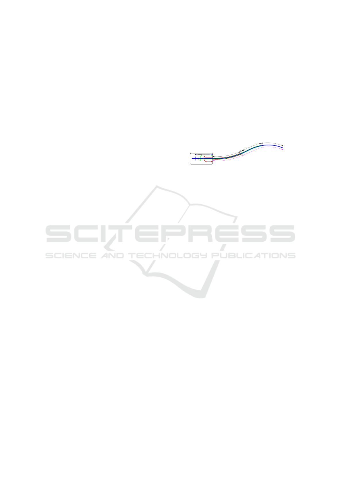
Figure 1: Schematic of the CTCR showing the notations
and controls.
2 MECHANICAL MODEL
The continuum robots addressed in this paper are as-
sumed to operate sufficiently slow, that the inertial ef-
fects are negligible. Therefore, the actual speed with
which the task performed is irrelevant and a quasi-
static model is used for the work. We assume per-
fectly elastic tubes, neglecting any possible hystere-
sis in the stress-strain relations. We also assume that
no external forces act on the robot along its length
or tip. A N-tubed CTCR consists of N concentric
tubes of lengths l
1
≥ · ·· ≥ l
N
, with the innermost tube
being the longest. The different lengths l
k
partition
any configuration into N segments S
k
each of length
L
k
:= l
k
− l
k+1
≥ 0 with the property each S
k
consist-
ing of k overlapping concentric tubes. The different
lengths l
k
partition the total length into N segments S
k
of length L
k
= l
k
− l
k+1
≥ 0 such that S
k
consists of k
concentric tubes for k = 1,.. .,N as shown in Figure 1.
For computational simplicity, the tubes for s < 0 are
considered with the angular feeds at s = 0 and there-
fore, corresponds to the actual actuator feeds given by
the operator. The section S
N
is located at the proximal
end and S
1
is present at the distal end. The inner-
most tube of length l
1
with material frame in its refer-
ence state is considered as backbone reference for our
formulation and computations. The relative rotation
of the constituent tubes about the common tangent
is measured with respect to this reference. The con-
figuration of the CTCR backbone (i.e., the innermost
tube) is described as an orientable curve in 3D space
described as a function of the arclength s ∈ [0, l
1
] us-
ing a centerline r : [0,l
1
] → R
3
and an attached or-
Navigation of Concentric Tube Continuum Robots using Optimal Control
147

thonormal director frame
R(s) = [d
1
(s),d
2
(s),d
3
(s)] ∈ SO(3), (1)
where the axes of the moving frame called directors
d
i
(s) ∈ R
3
are the columns of R(s). We derive the
equilibria explicitly in terms of position vector r(s)
and quaternions q(s) as a system of ODEs in a simi-
lar manner of Hamiltonian Formulation of rods (Dich-
mann et al., 1996). Quaternions or Euler parameters
q(s) ≡ (q
1
,q
2
,q
3
,q
4
) : [0,l
1
] → S
4
of unit length, i.e.,
|q(s)| = 1 are used in this model. They characterize
the director frame R(s) by
d
1
(s) =


q
2
1
− q
2
2
− q
2
3
+ q
2
4
2(q
1
q
2
+ q
3
q
4
)
2(q
1
q
3
− q
2
q
4
)


, (2a)
d
2
(s) =


2(q
1
q
2
− q
3
q
4
)
−q
2
1
+ q
2
2
− q
2
3
+ q
2
4
2(q
2
q
3
+ q
1
q
4
)


, (2b)
d
3
(s) =


2(q
1
q
3
+ q
2
q
4
)
2(q
2
q
3
− q
1
q
4
)
−q
2
1
− q
2
2
+ q
2
3
+ q
2
4


. (2c)
For brevity, the dependence of q
i
, i = 1, . ..,4 on s
is omitted. The director d
3
-axis is aligned along the
tangent of the curve centreline for inextensible and
unshearable rods. The spatial evolution of the frame
with respect to the arclength s is described with the
help of the Darboux vector u : [0,l
1
] → R
3
through the
relations d
i
0
(s) = u(s)× d
i
(s),i = 1, 2, 3, where × de-
notes the cross-product in R
3
. The strain components
u(s) · d
j
(s) ≡ u
j
(s) are obtained from the quaternions
q(s) through the relation
u
j
(s) = 2B
j
q(s) · q
0
(s), j = 1,2,3, (3)
where B
i
are 4 × 4 skew symmetric matrices given by
B
1
=



0 0 0 1
0 0 1 0
0 −1 0 0
−1 0 0 0



,B
2
=



0 0 −1 0
0 0 0 1
1 0 0 0
0 −1 0 0



,
B
3
=



0 1 0 0
−1 0 0 0
0 0 0 1
0 0 −1 0



These matrices, acting on q ∈ R
4
, result in orthogo-
nal vectors for i 6= j (i.e., B
i
q · B
j
q = 0) and give the
quaternion length when i = j as B
i
q · B
i
q = kqk
2
= 1.
The tubes are considered to be uniform, inextensible,
unshearable and transversely constitutively isotropic
with stiffness matrix K
[i]
= diag(K
[i]
11
,K
[i]
11
,K
[i]
33
) and
precurvature ˆu
[i]
=
h
ˆu
[i]
1
, ˆu
[i]
2
, ˆu
[i]
3
i
T
. Each concentric
tube has a constant stiffness matrix K
[i]
along its
length. As a notational convenience, we use a specific
step function K
[k]
(s) to extend it to a zero function
beyond its length l
k
as
K
[k]
(s) =
(
K
[k]
, s ∈ [0,l
k
],
0, s ∈ (l
k
,l
1
].
(4)
Here, l
k
is the length of the k-th tube calculated from
s = 0 and is related to the lengths of the overlapping
regions L
i
as l
k
=
∑
N
i=k
L
i
. Let α
[i]
: [0,l
i
] → R, i =
2,... ,N be the relative angle of twist between the tube
i and the reference innermost tube (tube 1) and
R
z
(α) :=


cosα −sin α 0
sinα cosα 0
0 0 1


be the rotation matrix about the variable tangent
d
3
-axis. The minimization of the total strain en-
ergy (Rucker et al., 2010) of the system of concentric
tubes yields the shape
˜
u ∈ R
3
and effective stiffness
K
eff
of the CTCR backbone as
˜
u(s) = K
eff
−1
(s)
N
∑
i=1
K
[i]
(s)R
z
(α
[i]
(s))
T
ˇ
u
[i]
,
K
eff
(s) =
N
∑
i=1
K
[i]
(s),
(5)
with
ˇ
u
[i]
=
h
ˆu
[i]
1
, ˆu
[i]
2
, ˆu
[i]
3
− α
[i]0
(s)
i
T
. Finally, the
equilibrium configuration of the robot in terms of its
position vector r(s), quaternions q(s) and the relative
twist angle α
[i]
(s) is given by the following set of first
order ODEs
r
0
(s) = d
3
(s), in ]0,l
1
[,
q
0
(s) =
3
∑
j=1
˜u
j
(s)
1
2
B
j
q(s), in ]0,l
1
[,
α
[i]
0
(s) =
∑
i
j=2
β
[ j]
(s)
K
[1]
33
(s)
+
β
[i]
(s)
K
[i]
33
(s)
+ ˆu
[i]
3
(s) − ˆu
[1]
3
(s), in ]0,l
i
[,
β
[i]
0
(s) =
K
[i]
11
(s) ˆu
[i]
1
(s)
∑
i
j=2
K
[ j]
11
(s)
·
i
∑
j=1
K
[ j]
11
(s) ˆu
[ j]
1
sin

α
[i]
(s) − α
[ j]
(s)

!
,
in ]0,l
i
[,
(6)
for the i = 2, ..., N outer tubes. The term α
[1]
(s) = 0
by definition. The last two terms are the result of
Euler-Lagrange equations on the total elastic strain
ICINCO 2022 - 19th International Conference on Informatics in Control, Automation and Robotics
148

energy of the system and β
[i]
is the canonical momen-
tum conjugate to α
[i]0
and it gives the twist moment in
the i th tube. The boundary conditions are specified
in terms of alignment of the innermost tube frame and
relative rotation of the other tubes at the root as
r(0) = 0, q(0) = [0,0, sinθ
1
,cos θ
1
],
α
[i]
(0) = α
[i]
o
, β
[i]
(l
i
) = 0, i = 2, 3, ..N,
(7)
where the conditions on β
[i]
corresponds to natural
boundary conditions. The tube k is not present
for s > l
k
and hence it has no contribution for the
deformation of the backbone for s ∈ [l
k
,l
1
]. The
d
1
− d
2
plane of the reference tube (inner tube) at
the root (s = 0) coincides with the fixed laboratory
e
1
− e
2
plane. The angle θ
1
corresponds to the
angle of rotation of the reference frame of inner tube
about e
3
≡ d
3
-axis at s = 0 and is controlled by the
user. The shape (r, q) must be continuous across the
boundary between the sections without any kinks.
The robot is controlled by varying the lengths L
i
of the segments, i.e., the feed of the tubes, and by
varying the initial conditions on α
[i]
o
, i.e., the rotation
of the tubes at the root. Note that any discretization
needs to take the coefficient discontinuities at the
segment boundaries l
i
into account for achieving the
nominal approximation order, e.g. by positioning grid
points at the segment boundaries or by formulating
the boundary value problem as a sequence of smaller
boundary value problems coupled by appropriate
boundary conditions. The latter approach is followed
here.
By solving the boundary value problem (6)–(7),
the equilibrium configuration of the robot i.e., its
r(y;s) and q(y;s) are obtained as a function of control
parameter vector y which is defined as
y := [L
1
,... ,L
N
,θ
1
,... ,θ
N
] ∈ R
2N
.
Here, θ
i
= θ
1
+ α
[i]
o
,i = 2,. ..,N is the angle of rota-
tion of the i-th tube. Thus, a CTCR with N tubes has
2N controls parameters determining its spatial config-
uration.
3 SYSTEM KINEMATICS
In the path planning task, the motion of the robot
is parameterized over pseudo-time t ∈ T := [0, 1],
since the actual speed of the motion is not relevant
in a quasi-static model. The control parameters y
at time t are written as y(t). A control rate vector
v(t) = [u
1
(t),. . .,u
N
(t),γ
1
(t),. . .,γ
N
(t)] and an initial
value y
0
are introduced to describe the system dynam-
ics defined as
˙
y(t) = v(t), y(0) = y
0
. (8)
The rates v
i
: T → R and γ
i
: T → R model the tra-
verse and rotational velocities of each tube, respec-
tively. The system dynamics (8) ensures the continu-
ity of control parameters on the whole time interval
T . The control parameters corresponding to the rota-
tion of the tubes, i.e., θ
i
,i = 1,... , N can take any real
value (being 2π-periodic), whereas the feed parame-
ters L
i
,i = 1,..., N can take only non-negative values
and are bounded by the maximum length of the tubes
L
i,max
resulting in the inequality constraint,
0 ≤ L
i
(t) ≤ L
i,max
∀t i = 1, . ..,N. (9)
Elastic instabilities like snapping can occur in these
CTCRs resulting in the sudden release of elastic strain
energy (Gilbert et al., 2016). Such situations are
avoided by using tubes shorter than a critical length
L
crit
.
4 OBJECTIVE FUNCTIONS
The task of navigating a robot in the best way is quan-
tified in terms of some objective function to be mini-
mized. Here, we consider prototypical objective func-
tions describing simple tasks.
Target Position: The primary goal for most robot
tasks is to maneuver the robot such that its tip reaches
a target point r
tar
and orientation q
tar
at the final time
t = 1. Obtaining a configuration simultaneously satis-
fying the position and orientation requirements is not
always possible, especially with a small number of
tubes, say, N ≤ 3. This requirement is best included
in the objective as a final time penalty:
M
1
(y) := kr(y(1),l
1
) − r
tar
k
2
+λkq(y(1),l
1
) − q
tar
k
2
,
(10)
where λ is the weighing term useful for pri-
oritizing between tip’s position and orientation
with k · k the Euclidean norm. The robot state
r(y(t); s,t),q(y(t); s,t) is obtained after solving the
boundary value problem (6)–(7) with control parame-
ters y(t). Alternatively, reaching the target position
and orientation could be specified as equality con-
straints, but since many combinations of position and
orientation are not exactly achievable, this would ren-
der the optimization task infeasible. Thus, relaxing
this requirement in form of a deviation penalty in the
objective is an attractive strategy. An alternative tar-
get requirement is to specify only the desired tangent
Navigation of Concentric Tube Continuum Robots using Optimal Control
149

of the tip, i.e., d
3
(y(1),l
1
), instead of the whole ori-
entation. In this case, the condition is imposed only
on a single director instead of all three director axes,
leaving the freedom of rotations around the robot tip
tangent. As the directors are normalized, this can be
formulated as minimizing the scalar product of the di-
rector and a given target direction:
M
1
(y) := kr(y(1),l
1
) − r
tar
k
2
− λd
3
(y(1),l
1
)· (11)
Path Tracing: Some applications may require the
tip to follow a prescribed curve r
path
(t) and orienta-
tion n
path
(t). These problems are dealt by including a
Lagrange term in the objective function as
J
1
(y) :=
Z
1
0

kr(y(t),t) − r
path
(t)k
2
− λd
3
(y(t),l
1
) · n
path
(t)

dt.
(12)
Covered Volume: Minimizing the working volume
of the robot i.e., the space traversed by it when per-
forming a task, is another quantity of interest. There
are several ways in which the working volume could
be quantified. One possible solution is the accumu-
lated deviation from the reference Follow the Leader
configuration r(y
FTL
,s). To perform or initiate any
task, the robot tip has to reach an initial point through
a FTL strategy with control parameters y
FTL
and
move form this position to trace a desired path. We
take the r(y
FTL
,s) configuration as a reference and
measure the robot’s deviation from this configuration,
which yields a rough measure of the working volume.
The smaller the deviation from the reference is, the
lower the robot’s interference with the neighboring
tissues. The corresponding objective is
J
2
(y) :=
Z
1
t=0
Z
l
1
(t)
s=0
d

r(y
FTL
,s),r(y(t), s)

ds dt,
(13)
where d(
ˆ
r,r(s)) is the distance of r(s)) from the ref-
erence configuration
ˆ
r. This is defined as the distance
to the arclength projection, i.e.,
d(
ˆ
r,r(s)) = k
ˆ
r(s
0
)−r(s)k with
Z
s
0
σ=0
ˆ
r
0
(σ)dσ = s.
(14)
Note that in the FTL configuration the innermost tube
can be assumed to have an infinite length, such that
the FTL arclength always exceeds s and the projec-
tion (14) is well-defined. A closely related, but quan-
titatively different means to quantify the working vol-
ume of the robot is the area swept by the robot during
its navigation, which is given by
J
2
(y) :=
Z
1
t=0
Z
ΣL
i
(t)
s=0
r
0
(s,t) ×
∂
∂t
r
0
(s,t) ds dt. (15)
Regularization: In addition, the square of the L
2
-
norm of the v(t) vector is included as a regularization
term in the objective function to avoid high-frequent
instabilities,
J
3
(v) :=
Z
1
t=0
kv(t)k
2
dt.
Furthermore, the solution can also be subjected to
path constraints of the form
g
l
≤ g(Y,t) ≤ g
u
, (16)
where g ∈ R
g
is some objective function depending
on the robot’s state and control parameters. One pos-
sible example is maintaining bounds on the robot tip
orientation in a task.
In total, we define the objective as a linear com-
bination of the individual contributions discussed
above,
J(y, v) = λ
0
M
1
(y) + λ
1
J
1
(y) + λ
2
J
2
(y) + λ
3
J
3
(v).
Depending on the application, some of the objective
terms can be more important than others, and may
be emphasized by a corresponding selection of the
weights λ
i
. Thus, we obtain the optimal control prob-
lem
min
y∈H
1
(T ),v∈L
2
(T )
J(y, v) (17)
subject to equality constraints (8) and inequality con-
straints (9) and (16).
5 DISCRETIZATION
Solving the optimal control problem numerically re-
quires a combination of discretization and optimiza-
tion methods. We follow the discretize-then-optimize
approach, also known as the direct method, and dis-
cretize the optimal control problem (17) in pseudo-
time t and arclength s in order to translate the problem
into a Non-linear Programming (NLP) problem to be
solved (Nocedal and Wright, 2006; Betts, 2010). We
divide the time interval [0,1] into m sub-intervals at
time points 0 = t
0
< t
1
··· < t
m
= 1, in the simplest
case with equidistant steps of length t
i+1
−t
i
=
1
m
. The
objective function is then approximated on these time
intervals using the trapezoidal rule as
J
m
= λ
0
M
1
+
1
m
1
2
¯
j(0) +
m−1
∑
i=1
¯
j(t
i
) +
1
2
¯
j(1)
!
,
where
¯
j(t) = λ
1
J
1
+ λ
2
J
2
+ λ
3
J
3
. The state r(s),q(s)
of the robot is obtained for the controls y(t
k
) at the
time points t
k
by discretizing and solving the bvp
ICINCO 2022 - 19th International Conference on Informatics in Control, Automation and Robotics
150

Table 1: Parameters of the CTCR used in the examples..
Option Tube 1 Tube 2 Tube 3
Bending Stiffness K
[i]
11
(×10
4
N.mm
2
) 1.0 1.2 1.4
Torsion Stiffness K
[i]
33
(×10
4
N.mm
2
) 1.0/1.3 1.2/1.3 1.4/1.3
Precurvature vector (mm
−1
) [1/200,0,0] [1/125,0,0] [1/100,0,0]
Maximum Length (mm) 330 220 110
problem (6), (7) using suitable collocation methods
(Kierzenka and Shampine, 2008) converting the in-
finite dimensional problem to an algebraic equation
system. From the robot state, the objective func-
tions j(t
k
) are computed, where the integrals along the
robot’s length arising in (13) are approximated again
using the trapezoidal rule. The ODEs (8) in the sys-
tem dynamics are approximated using central differ-
ences as
y
i
(t
k+1
) − y
1
(t
k
)
t
k+1
−t
k
= v
i
(t
k+1/2
) (18)
for i = 0,. . .,m − 1 in terms of the pseudo-velocities
v
i
(t
k+1/2
). The direct discretization results in a non-
linear program with 4Nm variables and 2Nm equal-
ity constraints. This NLP problem can be solved nu-
merically using a variety of available methods. Di-
rect methods use gradient-based techniques for solv-
ing the NLP and they require the gradient information
of the objective function and constraints. As some
of the objective terms are functions of solutions of
the bvp, analytical derivatives are not readily avail-
able. Instead, derivatives can be obtained by algorith-
mic differentiation or approximated by simple finite
differences (Griewank and Walther, 2000). For sim-
plicity of implementation, we use forward difference
schemes. The gradients are computed using IVP fi-
nite difference scheme in a similar manner as that in
(Rucker and Webster, 2011) and then supplied in the
sub-routines.
6 NUMERICAL EXAMPLES
We demonstrate the proposed optimal control frame-
work using a 3-tube CTCR. The mechanical prop-
erties of the constituent tubes are given in Table 1.
We consider tasks like guiding the robot tip to a pre-
scribed point and guiding it to a prescribed orienta-
tion. These numerical examples are solved with Mat-
lab’s fmincon which uses an interior point algorithm
(Nocedal and Wright, 2006).
6.1 Minimum Working Volume
In the first example, we consider maneuvering the
robot tip to a specified point r
tar
. Here, the orien-
tation and the path of the tip r
path
(t) are not impor-
tant and not accounted for in the overall objective
i.e., λ = 0 in (10) and λ
1
= 0. The effectiveness of
the proposed minimum deviation objective in reduc-
ing the working volume is examined by comparing
the cases with λ
2
= 0,50 and 200. Fixed values of
λ
0
= 400 and λ
3
= 5 are used throughout this sub-
section. The curve corresponding to the follow-the-
leader configuration with controls y
FTL
= [0.5,0.5 +
π,0.5 + π,0.4, 0.6, 0.5] is used as reference or mean
curve, and for calculating the objective (13). An ini-
tial configuration corresponding to the control param-
eters y(0) = [0.5,3.64,3.84,0.4, 0.6, 0.5] is used for
all the examples and a target r
tar
= (−0.4,0.0,1.0)
are chosen. No path constraints (16) are considered
in this task. The solution consisting of states cor-
responding to the control parameters y(0) is given
as initial guess at all time steps t
k
∈ [0,1]. The op-
timization is carried out using these parameters and
states. The evolution of the robot configurations and
its control parameters y(t) in the time interval [0,1]
are shown in Figure 2.
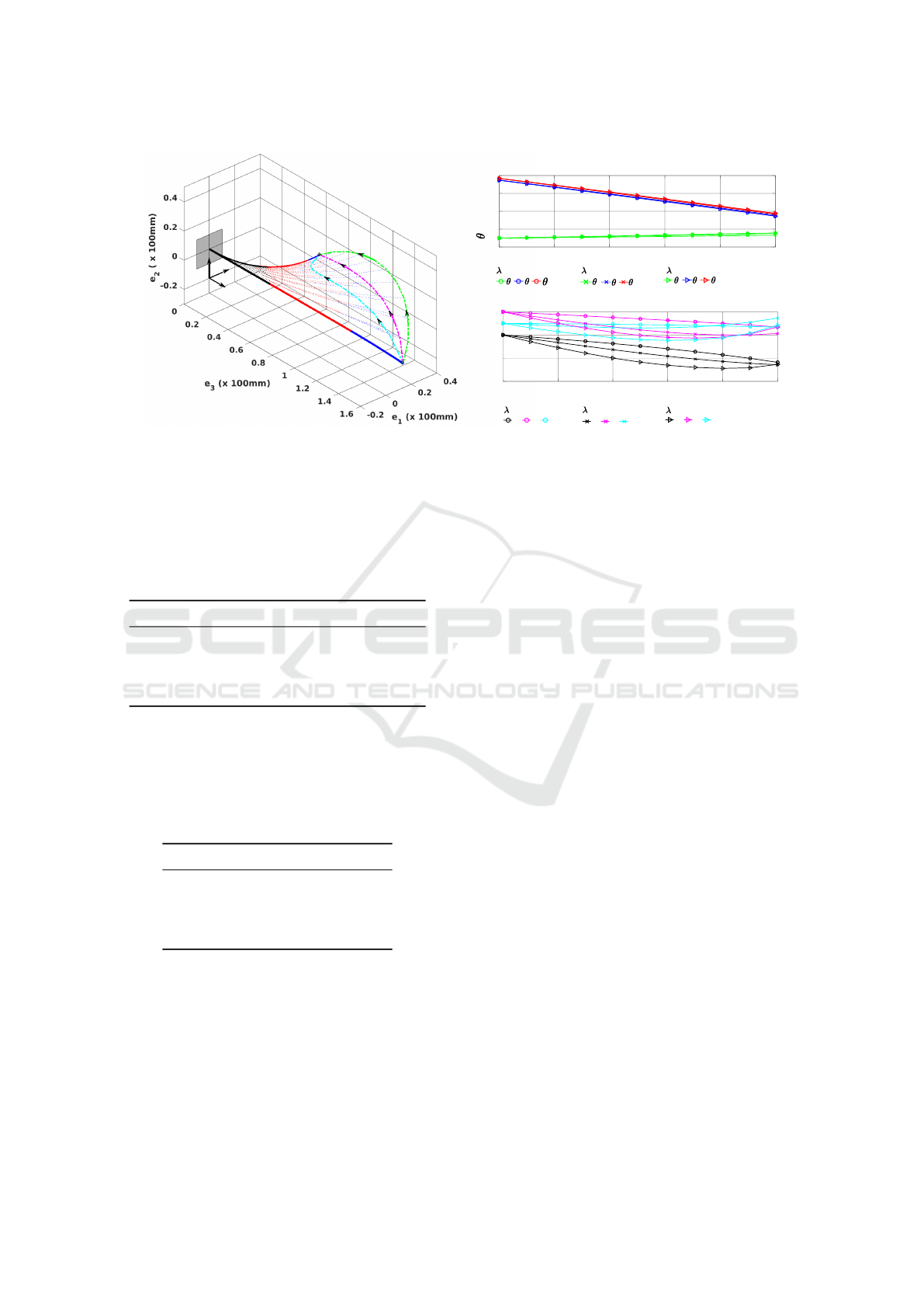
When the coefficient of the minimum deviation
measure J
2
, i.e. λ
2
is zero, the objective is to reach
the target r
tar
with the minimum regularization en-
ergy. As a result, the control parameters are obtained
as a linear function in the time interval [0,1] as can be
seen in Figure 2b. It appears qualitatively in Figure
2a that the robot occupies minimum working space
during a maneuver task for higher values of λ
2
and
is supported by the corresponding values of the de-
viation measure shown in Table 2. When the penalty
for the deviation term is non-zero, the robot navigated
with a minimum deviation path by reducing its length
in the period of its maneuver and extending its length
in the final period. These optimal solutions continu-
ously depend on the solution at initial time t = 0. The
obtained optimal solutions depend on the initial guess
and they vary if another initial guess is used.
The effect of using sweep area (15) as a minimum
volume measure is examined by comparing its values
Navigation of Concentric Tube Continuum Robots using Optimal Control
151

0 0.2 0.4 0.6 0.8 1
Time t
0
1
2
3
4
i
(t) (in rad)
Plot of rotation of tubes as a function of time t
1
2
3
=0:
1
2
3
=50:
1
2
3
=200:
0 0.2 0.4 0.6 0.8 1
Time t
0
0.2
0.4
0.6
L
i
(t) (x 100mm)
Plot of lengths of tubes as a function of time t
L
1
L
2
L
3
=0:
L
1
L
2
L
3
=50:
L
1
L
2
L
3
=200:
λ
2
=0
λ
2
=50
λ
2
=200
t=1
t=0
r
init
r
tar
e
2
e
3
e
1
a
b
Figure 2: (a) 3D views of the robot evolution with its tip r
tar
from r
int
with different penalization of volume minimization
objectives. The robot’s sections are shown in different colours with black, red and blue corresponding to sections with 3, 2,
and 1 tube, respectively. The trace of the tip is shown in green, magenta and cyan. The initial and final states of CTCR are
shown in solid lines whereas the intermediate states are shown in dotted lines. (b) The evolution of control parameters y(t)
for different λ
2
. The curves of rotation parameters θ
i
(t) for all cases of λ almost coincide. The markers correspond to the
mesh used for the computations. The control parameters at t = 1 for all three cases are different, but correspond to the same
tip point.
Table 2: Effect of the penalizing term λ
2
on the deviation
term (as calculated in (13) and the objective.
λ
2
Deviation term value J
2
Objective J
0 0.0544 20.4121
50 0.0220 21.8843
100 0.0162 22.8030
200 0.0107 23.9423
for different penalizing terms in Table 3. Increase of
the penalizing terms resulted in the decrease of the
sweep area measure J
2
, demonstrating the effective-
ness of the optimization framework.
Table 3: Effect of the penalizing term λ
2
on the sweep area
and the objective..
λ
2
Sweep area J
2
Objective J
0 0.4586 20.4121
5 0.2716 22.9218
10 0.2117 24.0679
20 0.1712 25.2532
6.2 Maintaining Fixed Tip Orientation
In this example, we include the tip orientation as well
as the target path r
path
(t) in the optimal problem. The
goal is to maneuver the robot tip close to a prescribed
path r
path
(t) with a restriction on the tip’s orienta-
tion d
3
(y(t),l
1
). The straight line between the ini-
tial point r
init
and the target r
tar
is specified as tar-
get path as r
path
(t) = (1 − t)r
init
+ tr
tar
∀t ∈ [0, 1].
The tip’s tangent of the initial state (t = 0) is taken as
n
tar
for this example. Therefore, the goal is to move
to the target r
tar
with minimum deviation of its tip’s
tangent from n
tar
. The penalization of the tip orien-
tation deviation is considered by using different val-
ues of λ. The minimum deviation objective J
2
is not
considered here: since the tip is constrained to move
along a path r
path
(t), its effect would be negligible.
λ
o
= 5, λ
1
= 400, λ
2
= 0, λ
3
= 5 are used in this ex-
ample. The time interval [0,1] is discretized into 10
equal intervals and 10 points on the straight line are
obtained. The evolution of robot and the angle be-
tween its tip tangent and the n
tar
for different values
of λ are plotted in Figure 3. However, not all specified
target points can be reached without violating the ori-
entation constraints. For such points, the robot does
not reach the specified point r
tar
. It gets to a posi-
tion as closer to r
tar
while satisfying the orientation
restriction.
6.3 Changing the Tip Orientation
without Changing Its Position
In the final example, we consider a task where the
robot tip is guided to a prescribed orientation n
tar
without changing its position. For this purpose, the
prescribed path in (12) is specified as a single point,
i.e., r
path
(t) = r
tar
. The optimization is carried out
by penalizing the deviation of the robot tip from the
target r
tar
. The penalizing terms λ
0
= 400, λ
1
= 100,
ICINCO 2022 - 19th International Conference on Informatics in Control, Automation and Robotics
152

Z
X
Y
R
init
R
tar
Angle between the target vector n
tar
the tip's tangent
(in °)
&
b
r
tar
r
init
t=0
t=1
e
3
e
1
e
2
a
0
0.2 0.4 0.6 0.8
1
Time t
0
2
4
6
8
10
12
14
Angle between the target vector and
the tip's tangent
(in °)
=0
=1
=1.5
=5
b
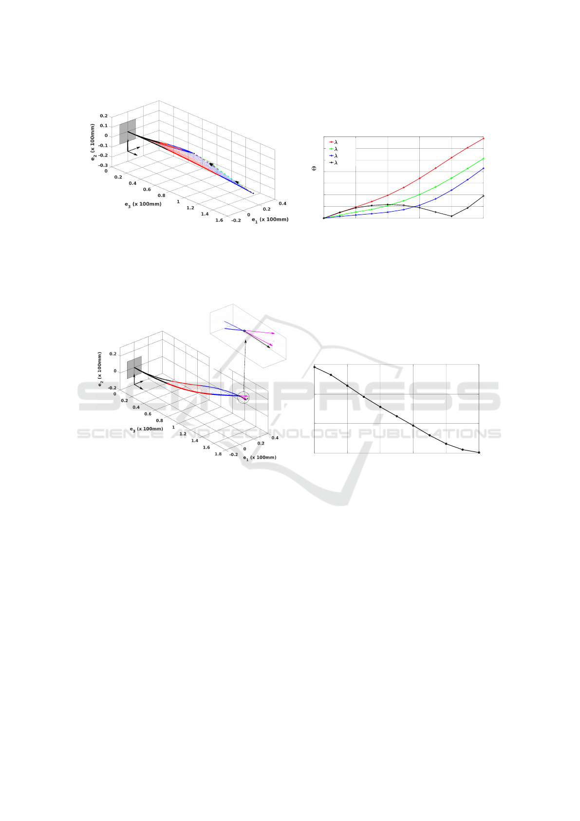
Figure 3: (a) The evolution of the CTCR as its tip moves from an initial point r
init
to a target r
tar
= [−0.01,0.12, 0.78]. The
tip is constrained to move along the straight line connecting r
init
and r
tar
by penalizing the deviation of the tip from the path.
The robot tip is guided closely to the specified target vector n
tar
by using non-zero penalization terms λ in (12). The traces of
the tip for different values of λ are shown. These traces are very close to each other. (b) The plots of the angle Θ between the
tip and the target vector n
tar
during the robot’s navigation for different values of λ.
0
0.2
0.4 0.6 0.8
1
Time t
5
10
15
20
Angle between the target vector n
tar
& the tip tangent Θ (in °)
r
tar
n
tar
e
3
e
1
e
2
t=1
t=0
r
tar
a
b
Figure 4: Example illustrating the maneuver of robot with its tip staying close to the initial tip point r
init
≡ r
tar
and the tip
tangent (in magenta) approaching the specified target n
tar
= [0,0,1]
T
(in black). The enlarged view of the region around the
tip is shown clearly indicating the tangents of the tip and the target n
tar
. The tip deviates slightly from the r
tar
during this
process. There is a slight difference of 5° angle between the tip’s tangent of the final state and the n
tar
at the final time (t = 1).
λ
2
= 0 and λ
3
= 5 are used for the implementation.
The configurations of the robot as its tip changes its
orientation to the target n
tar
= [0,0, 1]
T
, while its po-
sition staying close to the target r
tar
, are shown in
Figure 4. The tip’s orientation might not reach ev-
ery specified target orientation as configurations with
such orientation are not feasible. In such cases, the tip
just gets closer to the n
tar
and does not reach it.
7 CONCLUSIONS
Our work has presented a mathematical model for
guiding the robot in its workspace using optimal con-
trol techniques. The robot’s navigation is modelled
as a constrained optimal control problem and a suit-
able numerical strategy for its solution is described.
The numerical results suggest the usefulness of this
approach and show its potential for the application in
optimization based navigation tasks. The proposed
objectives, especially the minimum deviation objec-
tive, achieved the desired tasks and behaved qualita-
tively as expected. These objectives have conflicting
aims in some situations, where they were penalized
and degraded accordingly. The quaternion based state
equations are given in the simple compact form of the
first order ODEs and are useful for implementation
in any numerical package. The tip orientation has so
far been rarely considered in the literature, but ap-
pears to be useful for designing and planning more
complex tasks. In the current study, only unloaded
robots are considered. The given methodology can
Navigation of Concentric Tube Continuum Robots using Optimal Control
153

be extended from zero load to loaded cases after us-
ing the state equations from the geometrically exact
model (Rucker et al., 2010). The presented objectives
may have less conflicting effect on each other when
highly flexible CTCRs with more tubes are used. In
such situations, they have multiple configurations for
any required objective and the conflicting objectives
could find a compromise solution satisfying the re-
quirements. However, it is computationally complex
to solve problems with more than three tubes. Obsta-
cle avoidance can be considered by including the ob-
jective function (Lyons et al., 2009; Flaßkamp et al.,
2019) to the presented framework.
ACKNOWLEDGEMENTS
The research of Dhanakoti and Maddocks has been
funded by the Einstein Foundation Berlin.
REFERENCES
Alfalahi, H., Renda, F., and Stefanini, C. (2020). Concentric
tube robots for minimally invasive surgery: Current
applications and future opportunities. IEEE Trans.
Med. Robot. Bion.
Baykal, C., Torres, L. G., and Alterovitz, R. (2015). Opti-
mizing design parameters for sets of concentric tube
robots using sampling-based motion planning. In
2015 IEEE/RSJ International Conference on Intelli-
gent Robots and Systems (IROS), pages 4381–4387.
Bergeles, C., Gosline, A. H. C., Vasilyev, N. V., Codd,
P. J., del Nido, P. J., and Dupont, P. E. (2015). Con-
centric tube robot design and optimization based on
task and anatomical constraints. IEEE Transactions
on Robotics, 31:67–84.
Betts, J. T. (2010). Practical Methods for Optimal Control
and Estimation Using Nonlinear Programming, Sec-
ond Edition. Society for Industrial and Applied Math-
ematics, second edition.
Burgner, J., Rucker, D. C., Gilbert, H. B., Swaney, P. J.,
Russell, P. T., Weaver, K. D., and Webster, R. J.
(2013). A telerobotic system for transnasal surgery.
IEEE/ASME transactions on mechatronics : a joint
publication of the IEEE Industrial Electronics Soci-
ety and the ASME Dynamic Systems and Control Di-
vision, 19(3):996—1006.
Burgner, J., Swaney, P. J., Rucker, D. C., Gilbert, H. B.,
Nill, S. T., Russell, P. T., Weaver, K. D., and Webster
III, R. J. (2011). A bimanual teleoperated system for
endonasal skull base surgery. In 2011 IEEE/RSJ In-
ternational Conference on Intelligent Robots and Sys-
tems, pages 2517–2523.
Dichmann, D. J., Li, Y., and Maddocks, J. H. (1996).
Hamiltonian formulations and symmetries in rod me-
chanics. In Mesirov, J. P., Schulten, K., and Sumners,
D. W., editors, Mathematical approaches to biomolec-
ular structure and dynamics, pages 71–113. Springer.
Flaßkamp, K., Worthmann, K., M
¨
uhlenhoff, J., Greiner-
Petter, C., B
¨
uskens, C., Oertel, J., Keiner, D., and Sat-
tel, T. (2019). Towards optimal control of concentric
tube robots in stereotactic neurosurgery. Mathemati-
cal and Computer Modelling of Dynamical Systems,
25(6):560–574.
Garriga-Casanovas, A. and y Baena, F. R. (2018). Com-
plete follow-the-leader kinematics using concentric
tube robots. The International Journal of Robotics Re-
search, 37(1):197–222.
Gilbert, H. B., Hendrick, R. J., and Webster, R. J. (2016).
Elastic stability of concentric tube robots: A stabil-
ity measure and design test. IEEE transactions on
robotics : a publication of the IEEE Robotics and Au-
tomation Society, 32(1):20–35.
Gilbert, H. B., Neimat, J., and Webster, R. J. (2015). Con-
centric tube robots as steerable needles: Achieving
follow-the-leader deployment. IEEE Transactions on
Robotics, 31(2):246–258.
Granna, J., Godage, I. S., Wirz, R., Weaver, K. D., Webster,
R. J., and Burgner-Kahrs, J. (2016). A 3-d volume
coverage path planning algorithm with application to
intracerebral hemorrhage evacuation. IEEE Robotics
and Automation Letters, 1(2):876–883.
Griewank, A. and Walther, A. (2000). Evaluating deriva-
tives - principles and techniques of algorithmic dif-
ferentiation, second edition. In Frontiers in applied
mathematics.
Kierzenka, J. A. and Shampine, L. F. (2008). A BVP solver
that controls residual and error. JNAIAM J. Numer.
Anal. Ind. Appl. Math, pages 1–2.
Lyons, L. A., Webster, R. J., and Alterovitz, R. (2009). Mo-
tion planning for active cannulas. In 2009 IEEE/RSJ
International Conference on Intelligent Robots and
Systems, pages 801–806.
Nocedal, J. and Wright, S. (2006). Numerical Optimization.
Springer.
Rucker, D. C., Jones, B. A., and Webster III, R. J. (2010).
A geometrically exact model for externally loaded
concentric-tube continuum robots. IEEE transactions
on robotics : a publication of the IEEE Robotics and
Automation Society, 26(5):769–780.
Rucker, D. C. and Webster, R. J. (2011). Computing Jaco-
bians and compliance matrices for externally loaded
continuum robots. In 2011 IEEE International Con-
ference on Robotics and Automation, pages 945–950.
Rucker, D. C., Webster III, R. J., Chirikjian, G. S., and
Cowan, N. J. (2010). Equilibrium conformations of
concentric-tube continuum robots. The International
Journal of Robotics Research, 29(10):1263–1280.
Yip, M. C., Sganga, J., and Camarillo, D. B. (2017).
Autonomous control of continuum robot manipula-
tors for complex cardiac ablation tasks. J. Medical
Robotics Res., 2:1750002:1–1750002:13.
ICINCO 2022 - 19th International Conference on Informatics in Control, Automation and Robotics
154