Household Structure Projection: A Monte-Carlo based Approach
Wei Ping Goh
1
, Shu-Chen Tsai
1
, Hung-Jui Chang
2
, Ting-Yu Lin
1
, Chien-Chi Chang
1
, Mei-Lien Pan
3
,
Da-Wei Wang
1
and Tsan-Sheng Hsu
1,∗
1
Institute of Information Science, Academia Sinica, Taiwan, Republic of China
2
Department of Applied Mathematics, Chung Yuan Christian University, Taiwan, Republic of China
3
Information Technology Service Center, National Yang Ming Chiao Tung University, Taiwan
Keywords:
Household Structure Projection, Monte-Carlo, Agent-based Simulation.
Abstract:
The kernel of an agent based simulation system for spreading of infectious disease needs a so called household
structure (HSD) of the area being simulated which contains a list of households with the age of each member
in the household being recorded. Such a household structure is available in a Census that is usually released
every 10 years. Previous researches have shown the changing of the household structure has a great impact on
disease spreading patterns. It is observed that the changing of the household structure e.g., the average citizen
ages and household size, is at a faster speed. However, serious infectious diseases, such as SARS (year 2002),
H1N1 (year 2009) and COVID-19 (year 2019), occur with a higher frequency now than previous eras. For
example, it would be bad to use HSD
2010
built using Census 2010 to simulate COVID-19. In view of this
situation, we need a better way to obtain a good household structure in between the Census years in order for
an agent-based simulation system to be effective.
Note that though a detailed Census is not available every year, aggregated information such as the number of
households with a particular size, and the number of people of a particular age are usually available almost
monthly. Given HSD
x
, the household structure for year x, and the aggregated information from year y where
y > x, we propose a Monte-Carlo based approach “patching” HSD
x
to get an approximated HSD
y
. To validate
our algorithm, we pick x and y = x + 10 which both Censuses are available and find out the root-mean-square
error (RMSE) between Census’s HSD
y
and generated HSD
y
is fairly small for x = 1990 and 2000. The
spreading patterns obtained by our simulation system have good matches. We hence obtain HSD
2020
to be
used in your system for studying the spreading of COVID-19.
1 INTRODUCTION
The corona virus disease 2019 (COVID-19) has been
around the world since late 2019. According to World
Health Organization (2022), COVID-19 has infected
over 400 million and killed nearly 6 million peo-
ple (World Health Organization, 2022). The num-
bers are still rising. Clinical trial reports and re-
searches show that available vaccines have high ef-
ficacy against symptomatic infection and viral vari-
ants (Voysey et al., 2021; Baden et al., 2021; Thomas
et al., 2021; Gilbert et al., 2022; Tregoning et al.,
2021). One of the most effective ways to let us get
back to the “normal” live as before is to increase the
vaccination coverage. While vaccine supply is still
limited, developing an effective vaccination strategy
∗
Corresponding author.
becomes an important work.
We try to use a stochastic agent-based simula-
tion called SimTW developed by (Tsai et al., 2010)
to find out the best vaccination strategy for Taiwan.
The mock population is the kernel of SimTW. Sim-
ulation results with a vaccination intervention strat-
egy using a mock population generated from Census
2010 may not be effective because of the dramatic
demographic changes over years (Lin et al., 2021).
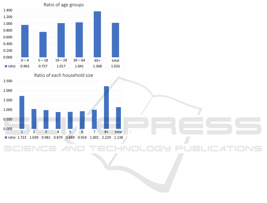
As shown in Figure 1, the population from 5 to 18-
year-old drop nearly 25% and the population above-
65-year-old is 36.8% higher comparing year 2010 and
year 2020. Moreover, the total number of households
has increased about 14%. The households contain-
ing 1 member, and 8 or more members have huge
increases. However, the number of households con-
taining 4 to 6 members are decreasing. An up-to-date
70
Goh, W., Tsai, S., Chang, H., Lin, T., Chang, C., Pan, M., Wang, D. and Hsu, T.
Household Structure Projection: A Monte-Carlo based Approach.
DOI: 10.5220/0011270100003274
In Proceedings of the 12th International Conference on Simulation and Modeling Methodologies, Technologies and Applications (SIMULTECH 2022), pages 70-79
ISBN: 978-989-758-578-4; ISSN: 2184-2841
Copyright
c
 2022 by SCITEPRESS – Science and Technology Publications, Lda. All rights reserved

mock population is highly needed in this research.
Census is carried out once per ten years, which leaves
the detailed information relevant to build a mock pop-
ulation lacking in non-Census years. However, some
high level aggregated data, such as the age distri-
bution and household statistics are available almost
yearly. Hence it is desirable to “patch” the mock pop-
ulation built from Census with recent updates.
Figure 1: The ratio of age groups and household size in year
2020 over year 2010.
A simulation approach to generate a household
structure distribution (HSD) with Census data, pro-
posed by Geard et al. (Geard et al., 2013), was used
in SimTW. This approach generates HSD for a given
mock population by a probability distribution over the
household patterns. The probability distribution of
the household pattern can be obtained from raw data
of Census released by (National Statistics, Taiwan, ).
Although the survey and report of Census 2020 were
done and released, the raw data are yet to be released.
To make sure having a relatively correct HSD and
age distributions at any specific year, we formulate
the probability distribution of the household pattern
building problem as a constrain satisfaction problem
and purpose a Monte-Carlo based method to solve it
using available aggregated data.
The structure of the rest of this paper is as follows.
In Section 2, we describe our data source and the sim-
ulation system we used. Then we describe the prob-
lem and our algorithms in Section 3. Section 4 will
describe the experimental design. In Section 5 and
Section 6, we show the validation and experimental
results. Finally, in Section 7, we give some discus-
sions and conclusions.
2 PRELIMINARY
In this section, we first describe related work and
method. Second, we introduce an agent-based sim-
ulation system called SimTW. Then we describe and
compare the data sources.
2.1 Related Work
Our needs can be said as a detailed version of the pop-
ulation projection problem (United Nations, 1946).
There are a total of 23 manuals and guides of de-
mographic related methods issued by the United Na-
tions (United Nations, 1946). Especially in Manual 1,
there are several methods and discussion about esti-
mating the total population in years later. This manual
states that the estimation based on incomplete enu-
merations and non-Census data are clearly more reli-
able than simply conjectures. In addition, six methods
including the arithmetic rate, the geometric rate, the
parabola of second/third degree and the second/third-
degree on logarithms are also given in this manual.
However, none of them are accurate in all aspects (UN
DESA, 1952). Manual IV also gives methods on esti-
mating demographic from aggregate and incomplete
data and also methods to appraisal the result (United
Nations, 1967). Also, several dimensions including
population size, educational attainment, etc..., need
to be considered when projecting the global popu-
lation (Lutz and KC, 2010). Methods of estimating
population based on grouping population by similar-
ity of fertility, mortality and migration are used in
multiple researches (United Nations, 1956; Gleditsch
et al., 2021). Research by (Dion, 2012) shows that
valid assumptions of the future proximate behavior
may lead to a better approximate result. These previ-
ous researches are classical but fail short to generate
the household structure we needed within regions of
a country.
2.2 Simulation System
SimTW is an agent-based stochastic and heteroge-
neous discrete time agent-based model developed in
(Tsai et al., 2010). This system uses a highly con-
nected network model representing daily interaction
between 23 million people living in Taiwan. Below is
a brief description of SimTW.
In this system, the entire population is classified
into five age groups, namely preschooler children (0-
Household Structure Projection: A Monte-Carlo based Approach
71

4 years old), school-age children (5-18 years old),
young-adults (19-29 years old), adults (30-64 years
old) and elders (65+ years old), which denoted as G
1
,
G
2
, G
3
, G
4
and G
5
respectively. In addition, each
family living together is tagged with the total num-
ber of people in the family and the number of people
in each age group. This family tag is called house-
hold pattern (HHP). An HHP, represents the number
of family members in each of the five age groups by
gender, and is encoded in five digits. These five digits
encode the number of members in each group from
elders to preschooler. For example, HHP = 20120,
is a household containing 2 elders, 0 adult, 1 young-
adult, 2 school-age children, 0 preschooler child. We
set an upper bound of no more than eight members
in any pattern for practical reason. Although there are
6
8
possible patterns, but there are only 18,176, 18,293
and 15,322 different patterns in Taiwan according to
Censuses 1990, 2000 and 2010 respectively. The
mock population of SimTW was built based on the
Taiwan Census Data at a granularity so called regions.
A region is a nature division of geographical area in
which people work and live. There are 368 regions in
the system and each region is characterized by an age
group distribution (AGD) which describes the number
of people in each age group, and a household structure
distribution (HSD) which are the numbers of HHP’s
among all possible HHP combinations.
The social structures were built based on (Ger-
mann et al., 2006) with local modification. A mix-
ing group is a daily close association of individuals,
where every member is connected with all other mem-
bers in the same group. The mixing groups in the
model can be divided into three categories: resident
areas, routine areas and surrounding areas.
Each simulation day is set as either workday, hol-
iday or long holiday according to the calendar pub-
lish by (DGPA, Taiwan, 2016). Each day is divided
into the daytime and night-time periods containing 12
hours each. During the daytime of a workday, indi-
viduals with work or studying go to their routine ar-
eas. During the night-time of workday and holiday,
only individual who commute to routine area go back
to the resident area and those who live in dormitory
remain in the routine area. Those who stay in dor-
mitories remain in routine area and they will go back
to their resident areas only during long holidays. All
individuals also active at the surrounding area in the
region where they stay.
SimTW uses the SEIR disease model as described
in (Krumkamp et al., 2011). There are two parame-
ters in this disease transmission model: contact prob-
ability (P
contact
) and transmission probability (P
trans
).
P
contact
represents the probability of an effective con-
tact between two individuals in a mixing group. The
details of P
contact
in each mixing group is derived from
a contact diary study of (Fu et al., 2012). P
trans
can be
said to be the infectivity of a pathogen when an effec-
tive contact occurs.
The model of FLU’s natural history in (Germann
et al., 2006) is used is this system. Latent period refers
to the time between E and I, in which the individual
does not have any symptoms or signs of infection,
while the incubation period is the time between in-
fection and symptom onset (Park and Ryu, 2018). In
this model, FLU’s average latent period, incubation
period and infectious period are 1.2 days, 1.9 days
and 4.1 days respectively. One-third of the infectious
individual appear to be asymptomatic.
2.3 Data Description
Data used in this paper can be classified in two cate-
gories: Census and household registration data. These
data both show the population status, but in different
ways.
Census data are collected from the Department
of Census, Directorate-General of Budget, Account-
ing and Statistics (DGBAS), Executive Yuan every 10
years. Census were done in Taiwan for more than
100 years. with the recent ones being in 1980, 1990,
2000, 2010 and 2020. Among them, 1980, 1990 and
2000 were conducted based on a complete enumera-
tion of residents but 2010 and 2020 were conducted
using sampling survey. Census contains detailed in-
formation and more accurate in “who is living in what
place”.
Household registration data are collected by the
Department of Household Registration, Ministry of
the Interior, Taiwan. There are a lot of population re-
lated data, for example gender and age distributions,
educational attainments, marital statuses etc ..., which
can be downloaded and used for understanding the
population statuses of Taiwan. These data are updated
and released every month. The household registration
data are records of “who registered in what place” for
regulations, which may not actually the place to live.
Although both data are not exactly the same, but
the population of each age group looks similar, with
a correlation coefficient of 0.997. We thus can con-
sider approximating the population distribution using
household registration data when the Census data is
not available.
SIMULTECH 2022 - 12th International Conference on Simulation and Modeling Methodologies, Technologies and Applications
72

Table 1: General convention of this paper.
Symbol Meaning
A
p
y
[r][i] general convention
A name of the main 2D array
y year
p
with p, it means a probability distribution
without p, its a number
r region index
i group index
C_A
y
Array A generated using Census data
R_A
y
Array A generated using Household
Registration data
M_A
y
Array A generated using PopuSet
H_A
y
Array A generated using an arithmetic
method based on HND
y
A_A
y
Array A generated using an arithmetic
method based on AGD
y
3 PROBLEM AND ALGORITHM
In this section, we first describe the notations and
definition used in this paper. Then we describe our
problem. Table 1 is the general convention used in
this work. HSD is a 2D array
HSD
y
= {(H
y
[1][1], H
y
[1][2], ··· , H
y
[1][n
HHP
]),
(H
y
[2][1], H
y
[2][2], ··· , H
y
[2][n
HHP
]), ··· ,
(H
y
[n
R
][1], H
y
[n
R
][2], ··· , H
y
[n
R
][n
HHP
])},
where n
HHP
is the total number of different HHP’s
and n
R
is the total number of regions. H
y
[r][i] is the
number of households with the ith HHP in the region
r. HHP is a 2D array
HHP
y
= {(T
y
[1][1], T
y
[1][2], · ·· , T
y
[1][n
AG
]),
(T
y
[2][1], T
y
[2][2], · ·· , T
y
[2][n
AG
]), · ·· ,
(T
y
[n
HHP
][1], T
y
[n
HHP
][2], · ·· , T
y
[n
HHP
][n
AG
])},
where n
AG
is the maximum number of age groups.
T
y
[i] denote the ith row which is the ith HHP pattern.
Each column represents an age group, and a number
in that column is the number of members in the
specific age group of that HHP pattern. Therefore,
T
y
[i][ j] is the number of members of household
pattern i in age group j. AGD is a 2D array
AGD
y
= {(A
y
[1][1], A
y
[1][2], ··· , A
y
[1][n
AG
]),
(A
y
[2][1], A
y
[2][2], ··· , A
y
[2][n
AG
]), ··· ,
(A
y
[n
R
][1], A
y
[n
R
][2], ··· , A
y
[n
R
][n
AG
])},
where A
y
[r][i] is the number of ith age group in the
region r. HND is a 2D array
HND
y
= {(N
y
[1][1], N
y
[1][2], ··· , N
y
[1][8]),
(N
y
[2][1], N
y
[2][2], ··· , N
y
[2][8]), ··· ,
(N
y
[n
R
][1], N
y
[n
R
][2], ··· , N
y
[n
R
][8])},
where N
y
[r][i] is the number of households com-
prising of i people, i ≤ 7, and N
y
[r][8] is the
number of households with 8 people or more in
region r. Let P(HND
y
[r]) be the probability dis-
tribution representation of HND
y
[r] which is the
array (
HND
y
[r][1]
|HND
y
[r]|
,
HND
y
[r][2]
|HND
y
[r]|
, ··· ,
HND
y
[r][n
i
]
|HND
y
[r]|
) where
|HND
y
[r]| =
∑
∀i
HND
y
[r][i]. P(HSD
y
[r]) can be
define in the same way. Thus P(HND
y
[r]) = N
p
y
[r] =
(N
p
y
[r][1], N
p
y
[r][2], · ·· , N
p
y
[r][8]) and P(HSD
y
[r]) =
H
p
y
[r] = (H
p
y
[r][1], H
p
y
[r][2], · ·· , H
p
y
[r][n
HHP
]).
Assume that year y is not a census year, but we
want to construct the household structure distribution
for year y. All we have from year y are the popula-
tion’s age group distributions (denoted by AGD
y
) and
household number distribution (denoted by HND
y
).
And we can look back to find closet Census year
x. For that year, not only C_AGD
x
, C_HND
x
and
C_HSD
x
are available. Using these available data,
we build M_HSD
y
. To validate, we can pick a cen-
sus year as y. And construct M_HSD
y
with our
method by assigning x as the previous census year.
Since C_HSD
y
exists, we then compare M_HSD
y
and
C_HSD
y
to get an idea of how good our algorithm is.
3.1 PopuSet
We have a detailed information published in Census
every 10 years, but only some aggregated monthly up-
dated information from other sources. The approach
we will be using is to generate a population model
every 10 years. Then an algorithm called PopuSet is
used to update the model by using the updated data
yearly. This section describes the algorithm PopuSet
we used to generate M_HSD
y
for year y.
The high level ideas of this algorithm is to revamp
C_HSD
x
to form M_HSD
y
using aggregated informa-
tion. First of all, we calculate the changes from year x
to year y with respect to the number of people in each
age group. We use δ
j
to denote the ratio of propor-
tion of age group j for different year. Using δ
j
, we
then calculate the estimated occurring probability of
HHP
i
among all household patterns in year y by mul-
tiplying the corresponding δ
j
’s. Hence the occurring
probability for ith HHP, can be estimated as H
p
y
[r][i]
= H
p
x
[r][i] ∗ Π
∀ j
δ
T
y
[i][ j]
j
. With the adjusted occurring
probability of each household pattern, H
p
y
[r][i], we
then adapt a Monte-Carol approach to generate each
household of a particular size one by one using the
occurring probability of H
p
y
.
In this algorithm, we first need to covert all the
data to fit the system format. After that we do a ba-
sic probability revamp based on the difference of the
populations. This step is called “basic/advanced” be-
cause it may need an advance revamp if the quality is
not good enough. Step 3 is the main part, we gener-
ate data iteratively until the constrains are met. The
last step is to check whether the quality of the gen-
Household Structure Projection: A Monte-Carlo based Approach
73

erated data good enough. If not, we go back to the
probability revamp step to do some advance revamp
then we repeat the above process until the quality is
acceptable. The detail of each step is describe below.
Algorithm 1: PopuSet.
Input: C_HSD
x
, C_HND
x
, C_AGD
x
;
R_HND
y
, R_AGD
y
.
Output: M_HSD
y
.
1: Initialization;
2: for all regions: do
3: Data conversion; (Algorithm 2)
4: repeat
5: Basic/Advanced Probability Revamp;
(Algorithm 3)
6: Iterative generating; (Algorithms 4)
7: Quality Checking; (Section 3.1.4)
8: until quality is acceptable
3.1.1 Data Conversion
The pseudo-code of this step is shown in Algorithm 2.
The purpose of this step is to convert existing data
into the format that fit to the system. Denote Pop[i]
the number of population in ith age group from data.
n
AG
is the number of age groups we need, n
PopD
is the
number of age groups from data. We declare an array
AGD that contain n
AG
value, then go through the data
for each age and then groups them as the specification
given.
Algorithm 2: Data Conversion.
Input: Pop[n
PopD
].
Output: AGD[n
AG
].
1: Initial: AGD[n
AG
] = {0};
2: for i = 1 to n
PopD
do
3: for j = 1 to n
AG
do
4: if i ∈ A[ j] then
5: AGD[ j] += Pop[i];  grouping the
population into its corresponding age group.
3.1.2 Basic/Advanced Probability Revamp
Algorithm 3 gives the detailed calculations needed to
it. For the basic revamping part, we adjust the proba-
bility according to the differences in the two data. The
revamped probability of each HHP (H
p
x
[i]) is equal to
the original probability times the difference in each
age group. If the quality of the generated data only
by the basic revamp is not good enough, then we use
an advanced revamp. The advanced revamp only ad-
justs few group types that not good enough. For ex-
ample we always lack of population in age preschool
children, it causes by the restrict of there is no house-
hold containing only preschool children. Thus it is
harder to add a new household containing multiple
members when each of the population in other groups
are fully allocated. We can do an advanced revamp
by adding an extra priority to the household contain-
ing preschool children. When we raised the probabil-
ities of all household containing preschool children,
the results get better.
Algorithm 3: Basic/Advanced Probability Revamp.
Input: C_HSD
x
[n
HHP
],C_HHP
x
[n
HHP
][n
AG
];
C_AGD
x
[n
AG
], R_AGD
y
[n
AG
].
Output: revamped C_HSD
x
[n
HHP
].
1: for j = 1 to n
AG
do
2: A
p
x
[ j] =
A
x
[ j]
|A
x
|
; A
p
y
[ j] =
A
y
[ j]
|A
y
|
;
3: δ
j
=
A
p
y
[ j]
A
p
x
[ j]
;  calculate the change of age
group j
4: for each possible HHP
i
, i from 1 to n
HHP
do
5: H
p
x
[i]∗ =
∏
n
AG
j=1
(δ
j
)
T
x
[i][ j]
;  revamp the
probability
3.1.3 Iterative Generating
The detail of the iterative generating process is shown
in Algorithm 4 There are multiple stages in this step.
Denote α
i
= (α
i
[1], α
i
[2], ··· , α
i
[8]) the weight for
refining the priority of R_HND
p
y
in stage i, β
i
=
(β
i
[1], β
i
[2], ··· , β
i
[8]) the target completion ratio of
R_HND
y
in stage i. We add a set of weight (α
i
) on
R_HND
p
y
in every stage to refine the priority of read-
ing which group first. We switch to the next stage
until a given conditions β
i
· R_HND
y
arrives. For ex-
ample the output result of the naive algorithm has a
low fitting rate on N
y
[6] to N
y
[8]. Then we use a two-
stages approach by picking HHP containing at least
6 members in the first stage and then the rest in the
second stage.
We start to generate M_HSD
y
with revamped
C_HSD
x
iteratively. Array AGD
0
y
is used to record the
allocated population in each age group. First, pick
a household size n based on R_HND
p
y
. A random
HHP containing n members is picked according to
the revamped C_HSD
p
x
. We then check if R_AGD
y
has enough quota to add. If yes, we add this HHP
into M_HSD
y
and reset the failure counter. Other-
wise, we increase the failure counter by 1 and then try
picking a new HHP. We set an upper bound n
try
to
prevent our program running forever.
SIMULTECH 2022 - 12th International Conference on Simulation and Modeling Methodologies, Technologies and Applications
74

Algorithm 4: Iterative Generating.
Input: revamped C_HSD
x
[n
HHP
], R_AGD
y
[n
AG
];
C_HHP
x
[n
HHP
][n
AG
], R_HND
y
[8].
Output: M_HSD
y
[n
HHP
].
1: Initial: AGD
0
y
[n
AG
] = {0}, HND
0
y
[8] = {0},
stage = 1, error = 0;
2: for stage = 1 to n
Stage
do
3: while error ≤ n
try
do  try until fail to add
any new HHP for n
try
times.
4: Random pick a number n based on
(α
stage
· R_HND
p
y
).
5: Random pick a HHP with the index h ac-
cording to revamped C_HSD
p
x
;
6: if ∀i, AGD
0
y
[i] ≤ R_AGD
y
[i] then
7: Add HHP
h
into M_HSD
y
.
8: for i = 1 to n
AG
do
9: AGD
0
y
[i] += T
x
[h][i];
10: HND
0
y
[n] ++;
11: error = 0;  reset error if successful.
12: else
13: error++;
14: if ∀ j, HND
0
y
[ j] ≥ (β
stage
· R_HND
y
[ j]) then
15: stage++;
3.1.4 Quality Checking
In the quality checking part, we calculate the popula-
tion and household composition’s weight root mean
square error (RMSE) between the generated and
household registration data to evaluate whether the re-
sult is good. The smaller the value is, the better the
result is. Define R(A, B) to be the RMSE of A over
B. As shown in Equation 1, we calculate RMSE of all
age groups in all regions using the formula below.
R(A, B)=
v
u
u
t
n
R
∑
i=1
n
i
∑
j=1
A[i][ j]
|A|
(
A[i][ j] − B[i][ j]
A[i][ j]
)
2
(1)
4 EXPERIMENTAL DESIGN
We have raw data from Census years 1990, 2000,
and 2010. Thus we can use the household distribu-
tion from previous Census to construct a household
distribution for next Census. Then compare the true
household structure distribution of the recent Census
year with our construction to validate our process. We
have two validations for M_HSD
y
, which are building
year 2000 from year 1990, and building year 2010
from year 2000 respectively. We also compare our re-
sults with the two published arithmetic based methods
(UN DESA, 1952). The first one is to do an arithmetic
adjustment based on age group distributions, and the
second one is based on household number distribu-
tions. A_HSD adjusted based on age group distribu-
tion is carried out in a way that is the same as the basic
revamp in Algorithm 3. H_HSD adjusted based on
household number distribution is calculated by Equa-
tion 2.
H
p
y
[r][i] = H
p
x
[r][i] ∗
N
p
y
[r][i]
N
p
x
[r][i]
(2)
Another evaluation approach is to compare the
simulated epidemic results. To catering to the sim-
ulation system SimTW, we construct the household
structure distribution for each region. We do not
make it explicit in the descriptions of the algorithms
to make the presentation clearer. Below is a recap
of the relevant parameters used in the simulation sys-
tem. The parameters that we use are as follows: The
system has a total of 5 age groups (n
AG
= 5). House-
holds containing 8 members is the largest household
in the system. The registration data have the popu-
lation age distribution from 0-year-old to above-100-
year-old (n
PopD
= 101). We set the maximum failure
limit n
try
= 50, 000.
We evaluate our results with two procedures. The
first is the detailed distribution of the mock population
generated by SimTW using those generated HSD
y
.
We show the average age, average household size
and the population distribution in the mock popula-
tions. Then we compare with RMSE’s of C_AGD
y
and C_HND
y
respectively. The second part is to com-
pare the simulation results with C_HSD
y
’s and from
generated HSD
y
’s. The simulation experiments in-
clude the two types of influenza virus. We choose
P
trans
= {0.08, 0.20} for those virus (denote as FLU
08
and FLU
20
respectively). The FLU
08
can be seen as
the A/H1N1 virus that first occurred at year 2009 in
Mexico (Bautista et al., 2010). FLU
20
roughly corre-
sponds to the SARS virus in year 2005 (Bauch et al.,
2005). The R
0
at years 2000, 2010 and 2020 all shown
in Table 2. The A/H1N1 virus occurred at years 2009
to 2010, with R
0
being 1.2 ∼ 1.4 according to the
(Dorigatti et al., 2012) research. The virus in others
year using the same P
trans
as the occurrence year but
having difference R
0
’s due to the difference in social
network and population compositions.
Table 2: R
0
of FLU
08
and FLU
20
from year 2000 to 2020.
Year FLU
08
FLU
20
2000 1.369 3.227
2010 1.306 3.047
2020 1.229 2.865
After validation, we then build M_HSD
2020
from
C_HSD
2010
which we aim for. We run SimTW using
Household Structure Projection: A Monte-Carlo based Approach
75

Table 3: Statistics of the mock population compare to with C_HSD
y
.
X_HSD
y
age
avg
size
avg
G
1
G
2
G
3
G
4
G
5
M_HSD
2000
1.002 0.973 0.997 1.000 1.000 1.000 1.001
H_HSD
2000
0.934 1.009 1.088 1.155 1.112 0.905 0.851
A_HSD
2000
0.884 1.195 1.134 1.309 1.104 0.866 0.694
M_HSD
2010
1.000 0.993 0.997 1.000 1.000 1.000 1.000
H_HSD
2010
0.914 1.005 1.420 1.163 1.187 0.898 0.809
A_HSD
2010
0.985 1.038 1.013 1.106 1.072 0.935 1.057
M_HSD
2020
and check whether the result is reason-
able.
5 VALIDATION
This section shows the validation processes. All sim-
ulation experiments have been performed 100 times
with the average result reported.
5.1 Statistics
Some of the basic statistics include average age
(age
avg
), average household size (size
avg
) and age
group distribution (G
1
∼ G
5
) using different models
are shown in Table 3.
From Table 3, we can see that M_HSD has good
results in both years 2000 and 2010. H_HSD and
A_HSD generated by arithmetic methods have some
significant differences. For example, the ratios of
school-age children are too high and those of elders
are too low for A_HSD
2000
. Furthermore, the ratios
for preschooler children are too high for H_HSD
2010
.
However, M_HSD fits the population distribution
well.
5.2 RMSE Comparison
In this section, we compare RMSE over C_HSD be-
tween M_HSD, H_HSD and A_HSD. As shown in
Table 4, M_HSD has the lowest RMSE over C_AGD
y
.
RMSE over C_HND
y
also has the lowest value in year
2010.
Table 4: RMSE of mock population compare with C_HSD
y
.
X_HSD
y
R(C_AGD,
X_AGD)
R(C_HND,
X_HND)
M_HSD
2000
0.015 0.082
H_HSD
2000
0.146 0.072
A_HSD
2000
0.216 0.502
M_HSD
2010
0.013 0.038
H_HSD
2010
0.190 0.081
A_HSD
2010
0.136 0.219
5.3 Simulation Result Comparison
In this section we further run the simulations with
all HSD’s generated using different approaches. We
compare all of the results by calculating the correla-
tion coefficient (CC) of the daily infected cases group
by group from G
1
to G
5
over C_HSD
y
. There are a
total of 16 simulation’s configurations, which are the
combinations of 2 diseases, 2 different years and 4
HSD’s generation approaches. The configuration of a
disease in year 20YY is denote as YY_DISEASE, for
example FLU
08
in year 2000 is denote as 00_FLU
08
.
We randomly add one index case every five days and
the duration of a simulation run is set at 930 days.
Note that in the rest of the paper, we may only show
data for a specific number of days and not all 930 days
for sake of simplicity.
The results with the configuration 00_FLU
08
are
shown in Table 5 and Figure 2(a). We can see
that the simulation using M_HSD
2000
has the high-
est CC results in all fields. Although the CC value
of H_HSD
2000
also has nice result, but there still
some significant differences when we compare the
daily infected cases. A_HSD
2000
shows a huge differ-
ence comparing to others because of a larger average
household size and a high ratio of school-age chil-
dren. H_HSD
2000
shows a better result comparing
with A_HSD
2000
, but also have a significant higher
front peak and an earlier second peak. M_HSD
2000
looks almost the same with C_HSD
2000
. Figure 2(a)
shows the daily infected cases.
Table 5: Correlation coefficient of all age groups based on
C_HSD
2000
using the configuration 00_FLU
08
.
00_FLU
08
G
1
G
2
G
3
G
4
G
5
M_HSD
2000
1.00 1.00 1.00 1.00 1.00
H_HSD
2000
0.94 0.95 0.96 0.94 0.93
A_HSD
2000
0.41 0.46 0.47 0.40 0.40
CC’s of other settings compared with C_HSD
2000
are shown in Table 6. M_HSD
2000
has value above
0.99 in all experiments at all fields. H_HSD
2000
and
A_HSD
2000
also have good CC results, especially for
FLU
20
. As shown in Table 2, all of the diseases hav-
SIMULTECH 2022 - 12th International Conference on Simulation and Modeling Methodologies, Technologies and Applications
76

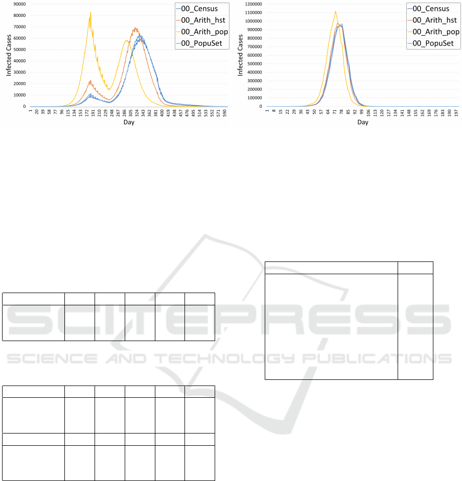
(a) FLU
08
(b) FLU
20
Figure 2: The daily infected cases of FLU
08
and FLU
20
at year 2000.
ing large R
0
’s lead to faster pandemics. That is, most
of the individuals are infected at early days which
shown in Figure 2(b). Even CC values are high, we
can still find that there are significant differences in
Figure 2(b). A_HSD
2000
always get a higher and
quicker pandemic at all experiments. PopuSet method
also has the best simulation result in the year 2010 as
seen in Table 7.
Table 6: Correlation coefficients of all age groups.
00_FLU
20
G
1
G
2
G
3
G
4
G
5
M_HSD
2000
1.00 1.00 1.00 1.00 1.00
H_HSD
2000
1.00 1.00 1.00 1.00 1.00
A_HSD
2000
0.93 0.93 0.94 0.93 0.92
Table 7: Correlation coefficients of all age groups in year
2010.
10_FLU
08
G
1
G
2
G
3
G
4
G
5
M_HSD
2010
0.99 0.99 0.99 0.99 0.99
H_HSD
2010
0.94 0.94 0.97 0.94 0.94
A_HSD
2010
0.75 0.76 0.84 0.76 0.74
10_FLU
20
G
1
G
2
G
3
G
4
G
5
M_HSD
2010
1.00 1.00 1.00 1.00 1.00
H_HSD
2010
1.00 1.00 1.00 1.00 1.00
A_HSD
2010
0.99 0.99 1.00 0.99 0.99
6 RESULT AND DISCUSSION
We demonstrate in Section 5 that PopuSet generates a
HSD
y
that is suitable for the simulation system when
R_AGD
y
and R_HND
y
are given. The raw data of
Census 2020 are not released, but the household reg-
istration data are available.
In this section, some statistics and simulation re-
sults of M_HSD
2020
are compared with R_AGD
2020
and R_HND
2020
as shown in Table 8. The ratio
of each age group fits well. The average age and
household size also fit well and both RMSE values
look good. Every ratio of whole population’s statis-
tic fits well and both R(R_AGD
2020
, M_AGD
2020
) and
R(R_HND
2020
, M_HND
2020
) look good, too.
Table 8: Statistics of M_HSD
2020
compare to with
R_HND
2020
and R_AGD
2020
.
Value
average age 1.000
average household size 0.995
preschooler children 0.996
school-age children 0.997
young adults 0.997
adults 0.997
elders 0.997
R(R_AGD
2020
, M_AGD
2020
) 0.030
R(R_HND
2020
, M_HND
2020
) 0.043
There are no C_HSD
2020
simulation’s result to
be compared with, but we can still compare with
C_HSD
2000
and C_HSD
2010
to check if the trend
looks reasonable. Figure 3 shows the simulation’s
result group by all diseases mentioned in Section 4.
We can see that the pandemic become milder. The
facts that a smaller household size and an aging soci-
ety both lead to a smaller pandemic (Lin et al., 2021;
Chang et al., 2015), we conclude that the trend of the
simulation’s results look reasonable.
7 CONCLUSIONS
We have shown a method called PopuSet to gener-
ate an approximated household structure based on the
existing household structure of previous Census and
yearly updated household registration data. This gen-
erated HSD
y
has better properties such as better fitted
population distributions and household sizes, compar-
ing with those generated by the arithmetic methods.
Household Structure Projection: A Monte-Carlo based Approach
77

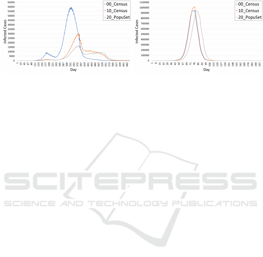
(a) FLU
08
(b) FLU
20
Figure 3: The daily infected cases of FLU
08
and FLU
20
year 2000, 2010 and 2020.
Take SimTW as an example, the mock population has
a great impact to the simulation result, but it can only
be updated every ten years from a costly Census sur-
vey. PopuSet performs some kinds of “update” every
year to C_HSD
y
.
We note that PopuSet can use some further im-
provements, especially when SimTW is simulating
diseases with R
0
≈ 1. The picking order of smaller
or larger households, the revamping strategy of prob-
ability are some of the parts that can be improved and
reasonable conjecture or heuristic may help. More re-
lated data and insightful information from data also an
important way to improve. We currently do not have
updates of information on worker and student flows
in aggregated forms. Without those data, the chang-
ing in social network cannot be updated. Our current
approach is to extrapolate linearly which may not be
a good practice when the societal structure, such as
rapid aging, and social interaction, such as the aver-
age household size, are changing in a very fast pace.
ACKNOWLEDGEMENTS
We thank Center for Survey Research (SRDA),
RCHSS, Academia Sinica, Taiwan for providing data
of Taiwan Census 2000 and 2010. This study was
supported in part by MOST, Taiwan Grants 107-2221-
E-001-017-MY2, 108-2221-E-001-011-MY3, 109-
2327-B-010-005 and 110-2222-E-033-005, and by
Research Center for Epidemic Prevention - National
Yang Ming Chiao Tung University (RCEP-NYCU).
REFERENCES
Baden, L. R., El Sahly, H. M., Essink, B., Kotloff, K., Frey,
S., Novak, R., Diemert, D., Spector, S. A., Rouphael,
N., Creech, C. B., et al. (2021). Efficacy and safety
of the mrna-1273 sars-cov-2 vaccine. New England
Journal of Medicine, 384(5):403–416.
Bauch, C. T., Lloyd-Smith, J. O., Coffee, M. P., and
Galvani, A. P. (2005). Dynamically modeling sars
and other newly emerging respiratory illnesses: past,
present, and future. Epidemiology, pages 791–801.
Bautista, E., Chotpitayasunondh, T., Gao, Z., Harper, S.,
Shaw, M., Uyeki, T., Zaki, S., Hayden, F., Hui,
D., Kettner, J., et al. (2010). Writing committee of
the who consultation on clinical aspects of pandemic
(h1n1) 2009 influenza. clinical aspects of pandemic
2009 influenza a (h1n1) virus infection. New England
Journal of Medicine, 362(18):1708–1719.
Chang, H.-J., Chuang, J.-H., Fu, Y.-C., Hsu, T.-S., Hsueh,
C.-W., Tsai, S.-C., and Wang, D.-W. (2015). The im-
pact of household structures on pandemic influenza
vaccination priority. In SIMULTECH, pages 482–487.
DGPA, Taiwan (2016). Directorate-general of personnel
administration, executive yuan, taiwan. https://www.
dgpa.gov.tw/. Online; Accessed: 2022 May.
Dion, P. (2012). Evaluating population projections: Insights
from a review made at statistics canada. In Annual
meeting of the Population Association of America, San
Francisco.
Dorigatti, I., Cauchemez, S., Pugliese, A., and Ferguson,
N. M. (2012). A new approach to characterising
infectious disease transmission dynamics from sen-
tinel surveillance: application to the italian 2009–
2010 a/h1n1 influenza pandemic. Epidemics, 4(1):9–
21.
Fu, Y.-c., Wang, D.-W., and Chuang, J.-H. (2012). Rep-
resentative contact diaries for modeling the spread of
infectious diseases in taiwan.
Geard, N., McCaw, J. M., Dorin, A., Korb, K. B., and
McVernon, J. (2013). Synthetic population dynam-
ics: A model of household demography. Journal of
Artificial Societies and Social Simulation, 16(1):8.
Germann, T. C., Kadau, K., Longini, I. M., and Macken,
C. A. (2006). Mitigation strategies for pandemic in-
fluenza in the united states. Proceedings of the Na-
tional Academy of Sciences, 103(15):5935–5940.
Gilbert, P. B., Montefiori, D. C., McDermott, A. B., Fong,
Y., Benkeser, D., Deng, W., Zhou, H., Houchens,
C. R., Martins, K., Jayashankar, L., et al. (2022). Im-
SIMULTECH 2022 - 12th International Conference on Simulation and Modeling Methodologies, Technologies and Applications
78

mune correlates analysis of the mrna-1273 covid-19
vaccine efficacy clinical trial. Science, 375(6576):43–
50.
Gleditsch, R. F., Rogne, A. F., Syse, A., and Thomas, M. J.
(2021). The accuracy of statistics norway’s national
population projections. Technical report, Discussion
Papers.
Krumkamp, R., Kretzschmar, M., Rudge, J., Ahmad, A.,
Hanvoravongchai, P., Westenhöfer, J., Stein, M., Put-
thasri, W., and Coker, R. (2011). Health service re-
source needs for pandemic influenza in developing
countries: a linked transmission dynamics, interven-
tions and resource demand model. Epidemiology &
Infection, 139(1):59–67.
Lin, T.-Y., Goh, W., Chang, H.-J., Pan, M.-L., Tsai, S.-
C., Wang, D.-W., and Hsu, T.-S. (2021). Changing
of spreading dynamics for infectious diseases in an
aging society: A simulation case study on flu pan-
demic. In Proceedings of the 11th International Con-
ference on Simulation and Modeling Methodologies,
Technologies and Applications - Volume 1: SIMUL-
TECH,, pages 453–460. INSTICC, SciTePress.
Lutz, W. and KC, S. (2010). Dimensions of global popula-
tion projections: what do we know about future pop-
ulation trends and structures? Philosophical Trans-
actions of the Royal Society B: Biological Sciences,
365(1554):2779–2791.
National Statistics, Taiwan. Directorate General of Bud-
get, Accounting and Statistics (DGBAS) of Execu-
tive Yuan. https://eng.stat.gov.tw/. Online; Accessed:
2022 May.
Park, J.-E. and Ryu, Y. (2018). Transmissibility and severity
of influenza virus by subtype. Infection, Genetics and
Evolution, 65:288–292.
Thomas, S. J., Moreira Jr, E. D., Kitchin, N., Absalon, J.,
Gurtman, A., Lockhart, S., Perez, J. L., Pérez Marc,
G., Polack, F. P., Zerbini, C., et al. (2021). Safety
and efficacy of the bnt162b2 mrna covid-19 vaccine
through 6 months. New England Journal of Medicine,
385(19):1761–1773.
Tregoning, J. S., Flight, K. E., Higham, S. L., Wang, Z., and
Pierce, B. F. (2021). Progress of the covid-19 vaccine
effort: viruses, vaccines and variants versus efficacy,
effectiveness and escape. Nature Reviews Immunol-
ogy, 21(10):626–636.
Tsai, M.-T., Chern, T.-C., Chuang, J.-H., Hsueh, C.-W.,
Kuo, H.-S., Liau, C.-J., Riley, S., Shen, B.-J., Shen,
C.-H., Wang, D.-W., and Hsu, T.-s. (2010). Efficient
simulation of the spatial transmission dynamics of in-
fluenza. PloS one, 5(11):e13292.
UN DESA (1952). Manuals on Methods of Estimating
Population-Manual 1: Methods of Estimating Total
Population for Current Dates. United Nations, De-
partment of Economic Affairs (UN DESA).
United Nations (1946). United nations demographic
manuals. https://www.un.org/en/development/desa/
population/publications/manual/index.asp. Online;
Accessed: 2022 May.
United Nations (1956). Manual iii. methods for population
projections by sex and age.
United Nations (1967). Manual iv: Methods of estimating
basic demographic measures from incomplete data.
Population Studies, 42.
Voysey, M., Clemens, S. A. C., Madhi, S. A., Weckx,
L. Y., Folegatti, P. M., Aley, P. K., Angus, B., Bail-
lie, V. L., Barnabas, S. L., Bhorat, Q. E., et al. (2021).
safetysafety and efficacy of the chadox1 ncov-19 vac-
cine (azd1222) against sars-cov-2: an interim analysis
of four randomised controlled trials in brazil, south
africa, and the uk. The Lancet, 397(10269):99–111.
World Health Organization (2022). Who coronavirus
(covid-19) dashboard. https://covid19.who.int/. On-
line; Accessed: 2022 Feb.
Household Structure Projection: A Monte-Carlo based Approach
79