Feature Extraction and Failure Detection Pipeline Applied to Log-based

and Production Data

Rosaria Rossini

1 a

, Nicol

o Bertozzi

1 b

, Eliseu Pereira

2 c

, Claudio Pastrone

1 d

and Gil Gonc¸alves

2 e

LINKS Foundation, Turin, Italy

SYSTEC, Research Center for Systems and Technologies, Faculty of Engineering, University of Porto, Porto, Portugal

Keywords:

Predictive Maintenance, Machine Learning, Feature Engineering, Manufacturing, Log Data, Drilling.

Abstract:

Machines can generate an enormous amount of data, complemented with production, alerts, failures, and

maintenance data, enabling through a feature engineering process the generation of solid datasets. Modern

machines incorporate sensors and data processing modules from factories, but in older equipment, these de-

vices must be installed with the machine already in production, or in some cases, it is not possible to install

all required sensors. In order to overcome this issue, and quickly start to analyze the machine behavior, in

this paper, a two-step log & production-based approach is described and applied to log and production data

with the aim of exploiting feature engineering applied to an industrial dataset. In particular, by aggregating

production and log data, the proposed two-steps analysis can be applied to predict if, in the near future, I) an

error will occur in such machine, and II) the gravity of such error, i.e. have a general evaluation if such issue

is a candidate failure or a scheduled stop. The proposed approach has been tested on a real scenario with data

collected from a woodworking drilling machine.

1 INTRODUCTION

Industry 4.0 paradigm aims to improve the plant level

of a factory by the means of different technology as-

sets, such as Internet of Things (IoT) sensors, Arti-

ﬁcial Intelligence (AI), data integration and aggrega-

tion, and so on and so forth. Industry 4.0 brings the

advantage of knowing better and in detail both pro-

cesses and machines involved in the production. This

advantage creates the possibility to not only know-

ing and monitoring the plant but also to improve the

process as well as the life and the work of the ma-

chine. In this context, RECLAIM

positions itself as

a project that has the goal to increase productivity, ex-

tending the lifetime of the machines and reducing the

time and cost of machinery refurbishment and/or re-

manufacturing. This objective will be achieved de-

signing and developing a set of tools supporting sev-

https://orcid.org/0000-0003-2029-7086

https://orcid.org/0000-0003-2049-9876

https://orcid.org/0000-0003-3893-3845

https://orcid.org/0000-0003-0471-8434

https://orcid.org/0000-0001-7757-7308

https://www.reclaim-project.eu/

eral activities: from the monitor of machines’ health

status, to the implementation of adequate recovery

strategy (e.g., refurbishment, re-manufacturing, up-

grade, maintenance, repair, recycle, and so on and so

forth). As RECLAIM shows, most of the time, it is

possible to improve the life of the machine and its

performance by improving the maintenance schedule

and/or manage the working time.

In order to do that, the authors present a two-steps

approach for machine diagnostics, based on log and

production data, that can predict and analyze the fail-

ures of the monitored machine. The goal is to apply

a pipeline with steps that include data cleaning, fea-

ture extraction, and predictive tasks to an industrial

dataset without using sensors data. After a prepro-

cessing step used to prepare the data and create the

input features, the classiﬁcation algorithm predicts is

a failure will happen in the next prediction windows

(PW), using the features present in the observation

windows (OW). The next component of the pipeline

is a severity estimation model that computes the level

of gravity of the predicted failure.

The strength, novel, innovative and convenient

aspect of this work is the possibility to do not in-

stall sensor data for the failure prediction, but using

320

Rossini, R., Bertozzi, N., Pereira, E., Pastrone, C. and Gonçalves, G.

Feature Extraction and Failure Detection Pipeline Applied to Log-based and Production Data.

DOI: 10.5220/0011268700003269

In Proceedings of the 11th International Conference on Data Science, Technology and Applications (DATA 2022), pages 320-327

ISBN: 978-989-758-583-8; ISSN: 2184-285X

only historical machine logs and production indica-

tors. In particular, the approach enables health mon-

itoring and the prediction of failures on older equip-

ment without the need of install new sensors. Those

attributes permit companies to reduce costs buying

new monitoring components and speeds the process

of analyzing the machine behavior and deploying the

predictive solution, because the monitoring system

(of log and production data) was on the machine since

the beginning of its operation generating historical

data.

The paper is organized as follows: in Section 2,

the authors introduce a literature review about predic-

tive maintenance and fault diagnosis. Section 3 de-

scribes brieﬂy the scenario in which the application

is described as well as the data available for it. Sec-

tion 4 presents the core solution presented in this pa-

per. Finally, Section 5 shows the results and Section 6

concludes the paper by summarizing and discussing

the work.

2 BACKGROUND

Nowadays modern machines are able to monitor a

large set of parameters, variables or indicators. The

production data is useful to build analytical solutions,

such as decision support systems or predictive main-

tenance solutions (Rosaria et al., 2021).

Among the operational data, machine failures and

alarms are some of the data sources most common in

the shop-ﬂoor. In fact, the PLCs continuously pro-

duce this log information about the machine, includ-

ing also internal events, warnings, alarms, errors, ma-

chine or components status or cycles. Logs are gen-

erated automatically at a very high rate, daily, hourly,

and contains timestamps about the information that is

reported. These log data can be stored into databases

or ﬁles, providing valuable information for machine

diagnostics (Xiang et al., 2018). Those diagnostics

algorithms can include degradation models or log-

based predictive maintenance (Gutschi et al., 2019),

(Wang et al., 2017). Despite of the structure of the

log ﬁle, managing these information can be an impor-

tant for extracting information about different aspect

of the machine production. As it is possible to see

in Section 3 log ﬁles can be also be involved in the

failure prediction.

3 DATASET

The data used for this work is from a woodworking

drilling machine described in detail in the subsection

3.1. That machine generates two different types of

data, 1) event log data, and 2) production data, which

are described in the subsection 3.2.

3.1 Scenario

The machine of interest is a woodworking drilling

machine (Brema VEKTOR15), composed of a set of

drill bits, divided into two spindles. The total number

of different drills is about 40/50. The life, in hours,

of a drill bit depends on multiple factors, such as the

hardness and wood quality. The quality of the mate-

rial depends on the suppliers and on what is indicated

in the speciﬁcations of the purchased wood. For in-

stance, the percentage of presence of metal residues

in the chipboards.

The shape of the drilled hole and the noise emit-

ted by the saw in case of cutting are good indicators

about the health of these tools. Due to the difﬁculty in

getting these measurements from the machinery, nor-

mally the drill bits are substituted or at regular inter-

vals or thanks to the operator’s experience.

3.2 Exploratory Data Analysis

The dataset used to design the pipeline is composed

of two parts: 1) the production data and 2) the log

data. The ﬁrst one contains all the articles produced,

and the second one all the events occurred in the ma-

chine. The extensions of those documents are .ter

and .btk, which are a particular type of text ﬁles, ex-

ported/generated by the machine.

3.2.1 Production Data

The production dataset, in Figure 1a, contains all the

pieces of wood worked in a particular time interval.

The description of the columns is the following: 1)

”Programma”, ﬁle that contains all the drilling opera-

tions that must be made on the piece, 2) ”Commento”,

details about the drilling, 3) dimensions of the board,

L for length, H for height, and S for width, and 4)

starting and ending time of the two working phases

(Start1, End1, Start2, End2).

One of the goals of this preliminary statistical

analysis is to evaluate to what degree of the working

time is inﬂuenced by the material (type of wood such

as poplar, ebony, walnut, etc.), the dimensions of the

board and the number of drills. A plausible starting

point is represented by the computation of derivative

variables like the volume, which integrates together

the length, the height and the width, and the time in-

tervals T1, T2 and INT. Instead, the value of T1 is the

difference, in seconds, between End1 and Start1, T2

Feature Extraction and Failure Detection Pipeline Applied to Log-based and Production Data

321

(a) Production data.

(b) Log data.

Figure 1: Dataset preview including machine production (a) and log data (b).

the difference between End2 and Start2 and, ﬁnally,

INT the difference between Start2 and End1.

The VEKTOR15 machine executes the drilling of

wood boards. Thus, the time required by the ma-

chine to perform those holes is linked to the number

of holes. In this view, variables T1 and T2 could be

directly connected to the number of operations per-

formed by the VEKTOR15, and consequently to the

product categories. Additionally, variables T1 are T2

are completely uncorrelated, which means that the

ﬁrst production phase does not give any information

about the time required by the subsequent stage.

3.2.2 Log Data

The log dataset, in Figure 1b, contains all the errors

emitted by the machine in a particular time interval.

The description of the columns is the following: 1)

timestamp of the error (time), 2) details about the er-

ror (description), 3) type, which includes three pos-

sible categories of error (Cycle, Done and System),

and 4) additional details about the error (Code, Task,

Status, ModAddr, Module, GroupCode).

In this case, the analysis is oriented to extract the

most serious stops, to retrieve a general pattern that is

speciﬁc-independent and to design a machine learn-

ing model that can predict future possible errors. The

only type of error that causes a stop of the machine is

the “System”. Then, all other logs can be discarded.

The available information about the speciﬁcations

of the error are in the ﬁeld “Description”. Summa-

rizing the description into a sentence with a reduced

number of words and without the redundant indica-

tion of the device numbers makes the analysis easier

and more interpretable. For instance, the error “XX: Il

servoazionamento YY non

e collegato” has a unique

error code, independently of the value of XX and YY.

After, the computation the ﬁnal list of errors includes

19 types of errors.

Figure 2a shows the entire production and the en-

tire generated log during 10 months of operation. It

is possible to notice that each production block is pe-

riodic, inline with the deﬁnition of a working week.

The space between each block represents a weekend.

Inside each block there are ﬁve smaller rectangles that

indicates a working day as well as in the ﬁrst two

weeks of August, due to the summer holidays, and in

some days over the year, due to the festivities. Last,

there is an absence of errors in some periods, e.g.,

February and May.

The distribution and the occurring time of the er-

ror is import and by observing the data, it is possible

to see that, multiple kind of errors (log samples with

different description/code) occur at the same time.

For our purpose, it is more important the chance of the

error to occur more than the type of error and, in a sec-

ond instance, the severity of it, i.e., its duration. The

machine learning models that will reach this goal will

be based on a set of production and error indicators,

trying to ﬁnd a causality between the time-production

and the insurgence of errors.

4 APPROACH

The analytical pipeline presented in this work, pre-

processes the data, extracting essential features from

both data sources (log events and production data),

computes observation, and prediction windows, and

feeds a binary classiﬁcation algorithm, that will pre-

dict if the class label of the current input sample is

equal to 1 (stop) or 0 (normal operation). In case of

a predicted stop, the model is triggered for the com-

putation of the severity (time to repair), that has four

levels of gravity.

4.1 Feature Extraction

Some of the features used to train the models are

the production indicators. Figure 3 shows the list of

the most produced categories in 9 months. The col-

umn “Count” indicates the number of drilled boards;

the “Ratio” reﬂects the percentage of production as-

signed to each category. From Figure 3, it is possible

to cover the 95% of production by summing only a

DATA 2022 - 11th International Conference on Data Science, Technology and Applications

322

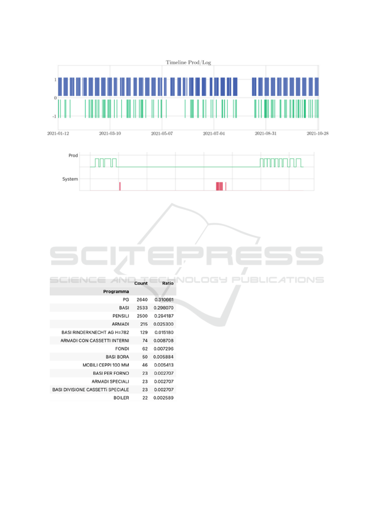
(a) Production and logs in the temporal line.

(b) Production and system errors in an extremely limited period of time, about 30 minutes.

Figure 2: Production and logs temporal line, with the entire period (a) and a period of 30 minutes (b).

small subset of categories, like “PG”, “BASI”, “PEN-

SILI”, “ARMADI”, and “BASI RINDERKNECHT

[...]”. This percentage is the threshold used to decide

which categories to include as features. After setting

these variables, the production indicators for each Ob-

servation Window (OW) include the cumulative num-

ber of drilled boards, together with the starting time

of the production.

Figure 3: Number of drilled boards for a subset of cate-

gories.

Figure 4 shows a typical subset of possible pro-

duction indicators with an OW with size 24,i.e, a tem-

poral window of 30 minutes. Each row of the produc-

tion dataset rapresents 12 working hours (the sum of

the preceding 24 row).

The log data pass through the same procedure, us-

ing a temporal region deﬁned precisely as the produc-

tion one. Given the number of errors in each window

(30 minutes), the cumulative sum is computed to de-

termine a historical characterization of the errors over

time. This approach allows the model to predict, con-

sidering the MTTF of each log category. The error

features are appended to the production ones as part

of the input of the classiﬁcation model. Those fea-

tures are essential for the classiﬁcation model because

stops and failures occur periodically or after a certain

number of produced articles.

The next step is to incorporate the working hours

and days into the prediction pipeline, allowing the op-

erational interpretation of the model results. For in-

stance, if at the 17:40 of a working day, the model pre-

dicts a failure in the next three temporal windows (1.5

hours) corresponds to a failure prediction for the ﬁrst

1.5 hours of production of the next day. Removing no

working hours and days is also essential to guarantee

a balancing between the classes labels in the dataset.

Usually, the working day begins at 6, included, and

ends at 18, excluded. Additionally, the intervals be-

tween 6-7, 12-13, and 17-18 are characterized by low

values of productivity and failures.

The number of errors and produced items allows

the computation of two metrics, that are essential to

evaluate the importance of each time interval: 1) the

sum of produced items and errors (PE indicator), and

2) the ratio of errors in the production (the number of

errors divided by the sum of errors and production)

(ER indicator). A low value of both indicators is a

Feature Extraction and Failure Detection Pipeline Applied to Log-based and Production Data

323

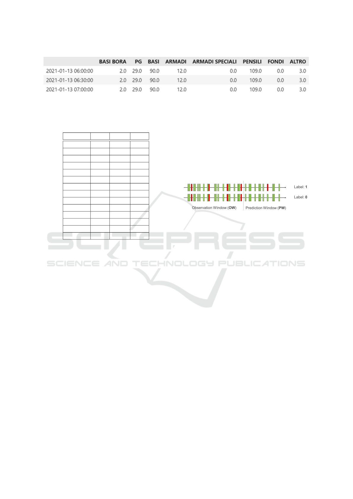
Figure 4: Example of some production indicators.

synonym of low interest in such time intervals.

Table 1: List of the working indicators for each hour.

Interval PE ER Risk

5-6 0 0 No

6-7 461 4.77 Yes

7-8 8308 32.64 Yes

8-9 8045 35.11 No

9-10 6401 37.45 No

10-11 9737 37.99 No

11-12 7912 32.42 No

12-13 276 0 Yes

13-14 6543 30.92 No

14-15 9519 47.31 No

15-16 8252 40.52 No

16-17 6608 44.87 No

17-18 816 57.72 Yes

18-19 0 0 No

Table 1 presents the values of the PE and ER in-

dicators. From the table, it’s possible to infer to 1)

drop the interval 12-13 due to the low value of PE and

ER, 2) maintain the interval 17-18 due to an extremely

high value of ER, and 3) consider if it is more conve-

nient to use also the samples contained in the interval

6-7, because of the lower value of PE and ER. The re-

moval of the interval 6-7 causes a drop in the model’s

precision mainly because the samples present in that

interval represent the initial base in predicting the fail-

ures of the next time intervals. The low values in the

interval 12-13 are due to the lunch break, which is not

zero because there are multiple lunch shifts; this also

supports the lower value of production in the interval

13-14.

The ﬁltering process also contemplates the not

working days. Those days include the summer hol-

idays and some festivities that cause the closure of

the plant and the consequent stop of production. In

addition, if some of these days fall on Tuesday or

Thursday, for instance, usually also the working days

near to the weekend, respectively Monday and Friday,

could be candidates for closure. Additionally, this ﬁl-

tering process permits lightening the unbalance of the

dataset.

4.2 Binary Classiﬁcation Model

The binary classiﬁcation model must predict if there

will be an error in the future time frame, given the

production, the actual time, and the historical list of

errors. The prediction model will implement a clas-

siﬁcation algorithm, where the class label equal to 1

corresponds to the prediction of failure in the future

time frame, and a class label of 0 to the normal oper-

ation of the machine (no failure).

Figure 5: Observation and prediction windows, with differ-

ent values of class label.

The prediction refers to a limited time slot, which

introduces the concepts of observation window and

prediction window. Figure 5 represents the two differ-

ent typical scenarios (prediction of failure or normal

behavior), where a temporal window is a ﬁxed-sized

period. The set of windows used to make a prediction

are the observation window (OW); the ones associ-

ated with the prediction form are the prediction win-

dow (PW). Then, given a series of OWs, the model

predicts if an error will occur between the actual time

and the end of the PW. The optimal conﬁguration is

characterized by a low value of PW because gives a

ﬁnal precision very conﬁned in time. However, this

introduces a trade-off between the precision (num-

ber of prediction windows) and the model’s perfor-

mance. So, to reach high performance, it is necessary

to forecast the error with low precision. The model re-

sults show that trade-off and compare different mod-

els with different values of OW and PW.

The classiﬁcation algorithms tested are the Ran-

dom Forest (RF) and the k-Nearest Neighbour (k-

NN). The RF has a good performance in classiﬁca-

tion problems. The k-NN performs well in clustered

samples, where the distance metric easily separates

the data samples. Looking at the samples distribu-

tion, considering the high level of isolation of label

items equal to 1, the suitable algorithm is the k-NN.

The hyperparameters are tuned for the entire pipeline,

including the preprocessing and the algorithm compo-

DATA 2022 - 11th International Conference on Data Science, Technology and Applications

324

nents. Regarding the preprocessing, the hyperparam-

eters to tune are the number of observing and predic-

tion windows, OW and PW, and the test size. For the

classiﬁcation model, the hyperparameters tested are

the number of estimators of the RF and the number of

neighbors of the k-NN. The approach used to the hy-

perparameter tuning was the k-fold cross-validation.

In datasets unbalanced, like this one, the adoption of

the accuracy as the evaluation metric is not ideal due

to the weight of the majority class. In this manner, due

to the high number of 0-labeled samples, the accuracy

can reach the same percentage of these samples con-

cerning the total number of rows of the dataset.

4.3 Stop Severity Estimation

The prediction of the error severity consists of esti-

mating the gravity of the VEKTOR15 stops and fail-

ures. The model presented provide information about

the gravity of the failure. The computed information

is useful to understand if the predicted stop will be a

short stop or a failure that causes the stoppage of the

machine for several days. Figure 6 illustrates a typi-

cal log cluster of a drilling machine. The production

samples have both the starting and the ending times-

tamp, while the log samples reported only the indica-

tion of the timestamp when the error occurred. For

this reason, it is not directly extracted from each clus-

ter of events an accurate value of duration or time to

repair (TTR) in case of failure. The log cluster in-

cludes the events (second row) between the produc-

tion interruption and its restart. The computation of

each cluster duration considers the ﬁrst event as start-

ing timestamp and the last one (restart of machine) as

the ending timestamp. In this way, it’s possible to ap-

proximate the stop duration and associate a severity

to each stop. There are four levels of failure severity,

1) no failure (label 0), and 2) three incremental values

of failure severity (labels 1, 2, and 3). The associa-

tion between the failure severity and the event clus-

ter duration is performed using different thresholds.

Those thresholds come from the 25th, 50th, and 75th

percentiles of the cluster duration distribution. The

subdivision in the percentage of labels is 30% label 1,

45% label 2, and 25% label 3, presenting all labels a

good value of balancing (close to 33%).

Figure 6: Deﬁnition of cluster duration. The faded orange

box indicates the uncertainty generated by the process.

Once each cluster has associated one severity

class, each temporal window has to be labeled de-

pending on the severity of the clusters it contains.

Windows containing more than one cluster, the label

associated is the one of the cluster with higher sever-

ity. After the computation of the new labels, the clas-

siﬁcation model passes through the same procedure

as the one done in binary classiﬁcation, being fed by

a series of OW and predicting the severity label of the

PW. The algorithms tested were the RF and the k-NN.

The binary classiﬁcation model and the stop severity

failure are complementary because they provide dif-

ferent indicators and are specialized in different tasks,

as show the results further ahead.

5 EXPERIMENTS & RESULTS

As mentioned before, the entire pipeline is tested

using the k-fold cross-validation. Different hyper-

parameters are experimented for both classiﬁcation

models and OW and PW.

5.1 Stop Detection Results

The f1-score is the used metric because it is the har-

monic mean of precision and recall and can be used

as a general indicator.

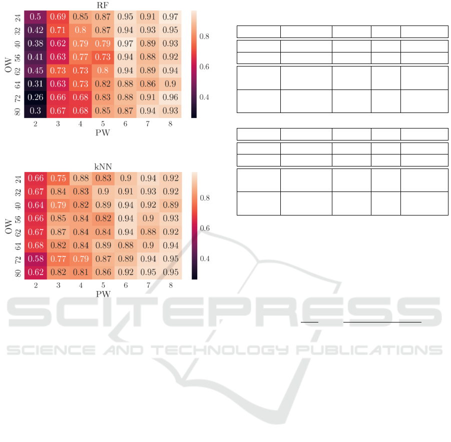
Figure 7 reports the results obtained with the Ran-

dom Forest and the k-Nearest Neighbour classiﬁer

with different observation and prediction windows.

The optimal classiﬁcation model will be the one that

reaches the best performance in terms of f1-score, re-

call, and with the lowest number of prediction win-

dows. Besides the number of PW, the decision crite-

ria between the different models instances will be the

arithmetic mean between the f1-score and the recall

of class 1. After analyzing Figure 7, it’s noticeable

that the pairs of (OW, PW) which satisfy the previous

objective function are (24, 4) for the RF and (62, 3)

for the k-NN.

Table 2 compares the two classiﬁers’ best results,

allowing the selection of the best one to be used in

production and on-site. Due to the high level of un-

balance, the indicators related to class 0 are not sig-

niﬁcant for that analysis. On the other hand, the re-

call, precision, and the f1-score of class 1 are more

meaningful. As mentioned before, the usage of those

metrics reduce false positives (FP) and false negatives

(FN).

It is observable that the k-NN results are slightly

better than the ones obtained by the RF because the re-

call is higher for the minority class (1-labelled), which

reduces the number of unpredicted failures (type II er-

ror). The level of f1-score is slightly lower in the k-

Feature Extraction and Failure Detection Pipeline Applied to Log-based and Production Data

325

(a) Results for the Random Forest (RF).

(b) Results for the k-Nearest Neighbour (k-NN).

Figure 7: F1-score results obtained by the Random Forest

(a) and k-Nearest Neighbour (b) in the binary case.

NN when compared to the RF; however, this decrease

is due to the higher precision of the RF. Since the type

I errors (false alarms) have less inﬂuence on the shop-

ﬂoor than the type II errors, the selected algorithm

should be the one with higher recall; even with a slight

decrease of f1-score. Additionally, using a higher ob-

servation window (OW) allows the model to consider

more historical information, including more failure

patterns. Those considerations imply that the k-NN

should be the selected classiﬁcation model to execute

on production because of the performance metrics and

the selected OW and PW.

5.2 Severity Prediction Evaluation

As in the binary task, the accuracy is not the ideal

performance metric for evaluating the severity model

due to the dataset imbalance. For this reason, the cor-

rective coefﬁcient used is the goodness (g) deﬁned in

Equation 1, where ˆy is the predicted class label, y the

real class label, and w the weights assigned to each

class. The goodness is adopted as corrective coef-

ﬁcient because the difference between the predicted

severity labels is crucial, i.e., it is not the equivalent

Table 2: Classiﬁcation reports obtained with the Random

Forest (a) and with the k-Nearest Neighbour (b).

Class Precision Recall F1 Support

0 0.98 0.99 0.99 625

1 0.90 0.84 0.87 67

macro

avg

0.90 0.84 0.87 692

weight

avg

0.97 0.98 0.98 692

(a) Random Forest results with OW=24 and PW=4.

Class Precision Recall F1 Support

0 0.99 0.98 0.99 633

1 0.81 0.89 0.85 53

macro

avg

0.90 0.93 0.92 686

weight

avg

0.98 0.98 0.98 686

(b) k-Nearest Neighbour results with OW=62 and PW=3.

predict a 0 or a 2 when the real class is equal to 3.

This situation reﬂects in the staff being prepared for a

small maintenance of the machine (predicted label 2)

or not being prepared at all (predicted label 2) when a

failure of high severity will happen (real label 1.)

g(y, ˆy, w) =

∑

i=1

∑

j=1

p( ˆy = i|y = j)

∑

j=1

p( ˆy = i|y = j)

(1)

A low value of goodness means a high level of

misclassiﬁcations; instead, a high value of goodness

indicates a minimal presence of critical situations like

the one described above. The classiﬁcation algo-

rithms experimented for this task were the k-NN and

RF, where the k-NN obtained better results than the

RF, practically for each pair of windows. Figure 8

reports the confusion matrices for the optimal conﬁg-

urations of OW and PW after applying the goodness

as the corrective coefﬁcient. As a correction coefﬁ-

cient, the goodness minimizes the distance between

the predicted severity and the real class. That effect

is noticeable in the confusion matrices, particularly

in the k-NN one, where the algorithm accurately pre-

dicted the severity of the failure almost every time.

So, the severity prediction model has an excellent per-

formance estimating the gravity of the stop; however,

it has lower performance when it comes to detecting if

it’s a failure or not (high number of FN and FP in the

label 0). That issue is addressed by using the binary

classiﬁcation model to predict if there is a stop or not,

and after, execute the severity model to estimate the

gravity of the expected stop.

DATA 2022 - 11th International Conference on Data Science, Technology and Applications

326

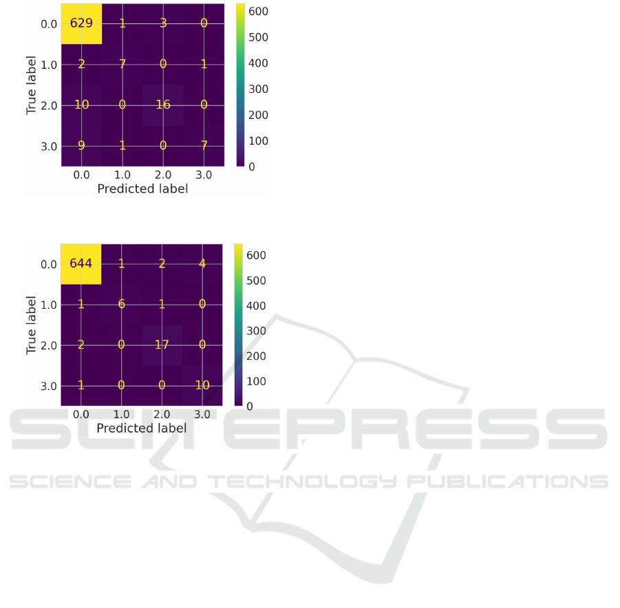
(a) Confusion matrix for the Random Forest (RF) with

OW=24 and PW=4.

(b) Confusion matrix for the k-Nearest Neighbour (k-NN)

with OW=62 and PW=3.

Figure 8: Confusion matrices obtained with the Random

Forest (a) and with the k-Nearest Neighbour (b).

6 CONCLUSIONS & FUTURE

WORK

The work in this paper developed provides a valu-

able pipeline for Prognostic and Health Management

(PHM). The pipeline was applied to a dataset gen-

erated by a woodworking drilling machine (Brema

VEKTOR15). That data includes machine log events

(alarms, stops, failures) and production data (pro-

duced pieces, including product type or working

time). The analytical pipeline preprocessed that data,

extracting essential features from both data sources,

computed observation, and prediction windows, and

feeding the binary classiﬁcation algorithm, which if

predicts a stop triggers the model for the computation

of the severity (time to repair). Those indicators pro-

vide essential information for the maintenance team,

mainly operational insights about when a failure will

occur and its impact. The usage of the severity model

provides essential insights to the operators because

it informs them if the predicted stop has a higher or

lower impact, which traduces in having a short stop

or the failure that could stop the machine for days.

The evaluation of the models results in the selec-

tion of the k-NN algorithm for the binary classiﬁer

(with OW=62 and PW=3) and severity predictor (with

OW=62 and PW=3). The excellent performance of

the k-NN for the two different tasks results from the

same input data that feeds each one of the models.

As future work, the goals pass through applying

the failure predictions (including severity) to deci-

sion support systems for the machine life and prod-

uct quality optimization. Another goal will be to val-

idate the algorithms using a simulation environment

that emulates the industrial shop ﬂoor. Finally, within

the project, it’s planned to apply this pipeline to other

industries like textile and white goods manufacturers.

ACKNOWLEDGMENT

The work presented here was part of the project

”RECLAIM- RE-manufaCturing and Refurbishment

LArge Industrial equipMent” and received funding

from the European Union’s Horizon 2020 research

and innovation programme under grant agreement No

869884. The authors thank PODIUM SWISS SA for

providing the data used in this paper and Asia Savino

for the support on data validation.

REFERENCES

Gutschi, C. et al. (2019). Log-based predictive main-

tenance in discrete parts manufacturing. Procedia

CIRP, 79:528–533. 12th CIRP Conference on Intelli-

gent Computation in Manufacturing Engineering, 18-

20 July 2018, Gulf of Naples, Italy.

Rosaria, R. et al. (2021). Ai environment for predic-

tive maintenance in a manufacturing scenario. In

2021 26th IEEE International Conference on Emerg-

ing Technologies and Factory Automation (ETFA ),

pages 1–8.

Wang, J. et al. (2017). Predictive maintenance based on

event-log analysis: A case study. IBM Journal of Re-

search and Development, 61(1):11:121–11:132.

Xiang, S., Huang, D., and Li, X. (2018). A generalized

predictive framework for data driven prognostics and

diagnostics using machine logs. In TENCON 2018 -

2018 IEEE Region 10 Conference, pages 0695–0700.

Feature Extraction and Failure Detection Pipeline Applied to Log-based and Production Data

327