Continuous Procedural Network of Roads Generation using L-Systems

and Reinforcement Learning

Ciprian Paduraru, Miruna Paduraru and Stefan Iordache

University of Bucharest, Romania

Keywords:

Networks, Roads, Deep Learning, Simulation Software, Video Games, L-systems, Reinforcement Learning.

Abstract:

Procedural content generation methods are nowadays used in areas such as games, simulations or the movie

industry to generate large amounts of data with lower development costs. Our work attempts to ﬁll a gap in this

area by focusing on methods capable of generating content representing network of roads, taking into account

real-world patterns or user-deﬁned input structures. At the low- level of our generative processes, we use

L-systems and Reinforcement Learning based solutions that are employed to generate tiles of road structures

in environments that are partitioned as 2D grids. As the evaluation section shows, these methods are suitable

for runtime demanding applications since the computational cost is not signiﬁcant.

1 INTRODUCTION

The environments used by computer games, simu-

lation applications, and movies have grown signiﬁ-

cantly in recent years. Nowadays, most users demand

large open-space worlds with lots of content. Proce-

dural content generation is currently used to generate

textures (Dong et al., 2020), animations (Danny Al-

berto et al., 2019), and virtual worlds (Freiknecht

and Effelsberg, 2017). Open-world games such as

Minecraft

, NoMansSky,

, the Far Cry series, or

movies such as The Mandalorian

use procedural

content generation to increase the size of environ-

ments and reduce production costs.

Our work addresses the problem of procedural

generation of road networks that bear a resemblance

to real cities. Our motivation stems ﬁrstly from the

set of applications that could use such a system, such

as simulators for self-driving cars, driving simulation

environments, and computer games. Second, after a

literature review, we ﬁnd that there is a gap in this

area. The contribution of our current work can be

summarized from two points of view:

• From the authors’ knowledge, this is the ﬁrst work

that builds generative models for networks of

https://www.minecraft.net/en-us

https://www.nomanssky.com/

https://www.theverge.com/2020/2/20/21145671/mand

alorian-sets-stagecraft-epic-games-ilm-fortnite-baby-yod

a-digital

streets that mimic real-world cities. Our methods

are based on statistical learning of features, which

are then sampled by L-Systems (Curry, 2000) or

training Reinforcement Learning (RL) agents to

generate the networks.

• Provide an augmented dataset and operations

where the road network pictures from different

real cities are converted into a graph format suit-

able for further research in the community. We be-

lieve that the methods and code used for process-

ing can be easily adapted to other inputs such as

maps from Open Street Maps

or Google Maps.

The contributions are also made open source at https:

//github.com/AGAPIA/ProceduralContentGeneratio

The rest of this paper is organized as follows. Sec-

tion 2 describes previous work on procedural content

generation, focusing on map generation. Section 3

presents the processing methods for converting top-

down pictures of cities into augmented graph struc-

tures. Our methods and procedural content generation

proccesses are described in Section 4. The evaluation

of our work is considered in Section 5. The ﬁnal sec-

tion contains a conclusion and plans for future work.

https://www.openstreetmap.org/

Paduraru, C., Paduraru, M. and Iordache, S.

Continuous Procedural Network of Roads Generation using L-Systems and Reinforcement Learning.

DOI: 10.5220/0011268300003266

In Proceedings of the 17th International Conference on Software Technologies (ICSOFT 2022), pages 425-432

ISBN: 978-989-758-588-3; ISSN: 2184-2833

425

2 RELATED WORK

Important content of the current top video games use

the so-called ’Procedural Content Generation’ (PCG)

to improve gameplay and make the game more inter-

esting and entertaining for players (Liu et al., 2020).

We will analyze some methods that have been used so

far in content generation, focusing primarily on map

generation. Dynamic map generation for video games

has been studied in many papers in the literature. In

this section we will try to describe the state of the art

in this ﬁeld and compare it with our current work.

L-Systems where used in (Parish and M

uller,

2001) to create procedural cities. Compared to our

method, their method is purely generative and re-

ceives as inputs goals and constraints and does not

learn a model from real data topologies. Tensor

ﬁelds were also used in (Chen et al., 2008), but with

the same drawbacks, since it is a purely generative

method based on constraints. In (Lara-Cabrera et al.,

2012), the authors use a genetic algorithm to gener-

ate and evolve balanced maps (i.e., maps that provide

equal advantages and disadvantages to all players) for

real-time strategy (RTS) games. Their method gener-

ates content ofﬂine using a generate-and-test schema.

The algorithm runs over a set number of generations

with a tunable population size, where each individ-

ual maps 84 different parameters. The selection pro-

cess is done in a tournament way and uses a mutation

rate of ∼ 70% and a crossover rate of 75%. To cal-

culate an individual’s score, a genotype-to-phenotype

transformation was used. Evaluating how balanced

a generated map is, it is a costly process where two

bots play the game until the end and evaluate the bal-

ance coefﬁcient. In (de Ara

ujo et al., 2020), Particle

Swarm Optimizations (PSO) techniques are used to

generate balanced maps that simultaneously satisfy a

set of soft user-speciﬁed requirements. Their method

assigns a particle to each tile of the map (which is

organized in a grid structure similar to our solution)

and penalizes each tile for deviating from the user-

suggested requirements. However, their generative

process uses random heuristics to some sense. Apply-

ing such methods to structures with constrained ge-

ometry, such as 2D graphs in our case, would lead to

poor results and lose the expressiveness of a real-life

example.

In (Snodgrass and Onta

on, 2017), a more sta-

tistical approach to content generation is presented

that uses multidimensional Markov Chains (MdMC)

to generate tiles of simple 2D levels in games. The

MdMC is trained using existing data and then sam-

pled to generate more content at runtime. Although

its approach is interesting for our purpose, it is lim-

ited to generating game levels where each tile could

deﬁne a piece in the world, which could not lead

to learning the structure of smooth roads in a city’s

road network. The same limitation is found in (Ping

and Dingli, 2020), which uses Conditional Generative

Adversarial Networks (cGAN) to generate 2D or 3D

maps based on a user-speciﬁed sketch. In addition,

this method needs the generation of a sketch of the

map ﬁrst, and it is difﬁcult to adapt it to a constantly

moving visualization perspective inside the environ-

ment.

An approach that uses reinforcement learning is

described in (Gissl

en et al., 2021). Their method con-

sists of two RL agents: the generator and the solver,

which are interdependent. The generator creates an

environment, which is then tested by the solver. The

generator receives feedback (rewards and observa-

tions) from the solver, as well as some additional con-

tent speciﬁed by the developers. In this way, the gen-

erator learns to create different types of environments

of varying types, difﬁculty, and complexity. After the

generator creates a new environment, it challenges the

problem solver to produce the best possible result. As

a result, the problem solver becomes more robust and

is more likely to solve new, unprecedented tasks and

reduce the amount of hard coding required to solve

the task. However, we note that the method is not suit-

able for our purposes because the computational cost

of generating new tiles with connected roads would

not be suitable for runtime generation.

Given our goal of learning graphs of networks

and then training a model that creates similar look-

ing graphs, an approach such as NetGAN (Bojchevski

et al., 2018) that uses Generative Adversarial Net-

works (GANs) could also be used. However, the

problem with NetGan is that it only supports undi-

rected graphs and cannot generate continuous net-

works as we need in a procedurally generated road

network. Another approach is Misc-GAN (Zhou

et al., 2019), where graphs are fed into a GAN ar-

chitecture that tries to extract a distribution for the

given graph dataset at different levels of granular-

ity. The network learns this distribution and then

attempts to apply it to the patterns being generated.

Like the previous approach, this method is not suit-

able for generating continuous road networks, only

individual samples, which is not of great use for our

goal. The work presented in GraphGAN (Wang et al.,

2017) and VGAE (Kipf and Welling, 2016) is de-

signed for datasets where the user deﬁnes the set of

nodes and the model can then ﬁll in the edges. How-

ever, our goal is to generate both nodes and edges,

which means that the approach they use is not suit-

able for our requirements. We try to overcome these

ICSOFT 2022 - 17th International Conference on Software Technologies

426

limitations with our proposed solutions based on re-

inforcement learning.

3 DATASET AND PROCESSING

ALGORITHMS

To model a generative method that learns from real

data, we will use the semantic representation of the

CITY-OSM dataset (Li et al., 2019). The dataset con-

sists of 1671 aerial images of the cities of Berlin,

Chicago, Paris, Potsdam, Tokyo, and Zurich, which

together comprise nearly 45 GB. The raw images

were segmented into a simpler representation consist-

ing of roads (marked with the color blue RGB(0, 0,

255)), buildings (marked with the color red RGB(255,

0, 0)), and the rest of the background (marked with

the color white RGB(0, 0, 0)). Note that similar input

content can be added by computer vision methods di-

rectly from Open Street Map or Google Maps. There-

fore, we believe that the methods described below are

also suitable for customized and new input maps.

3.1 Detecting Road Nodes and Edges

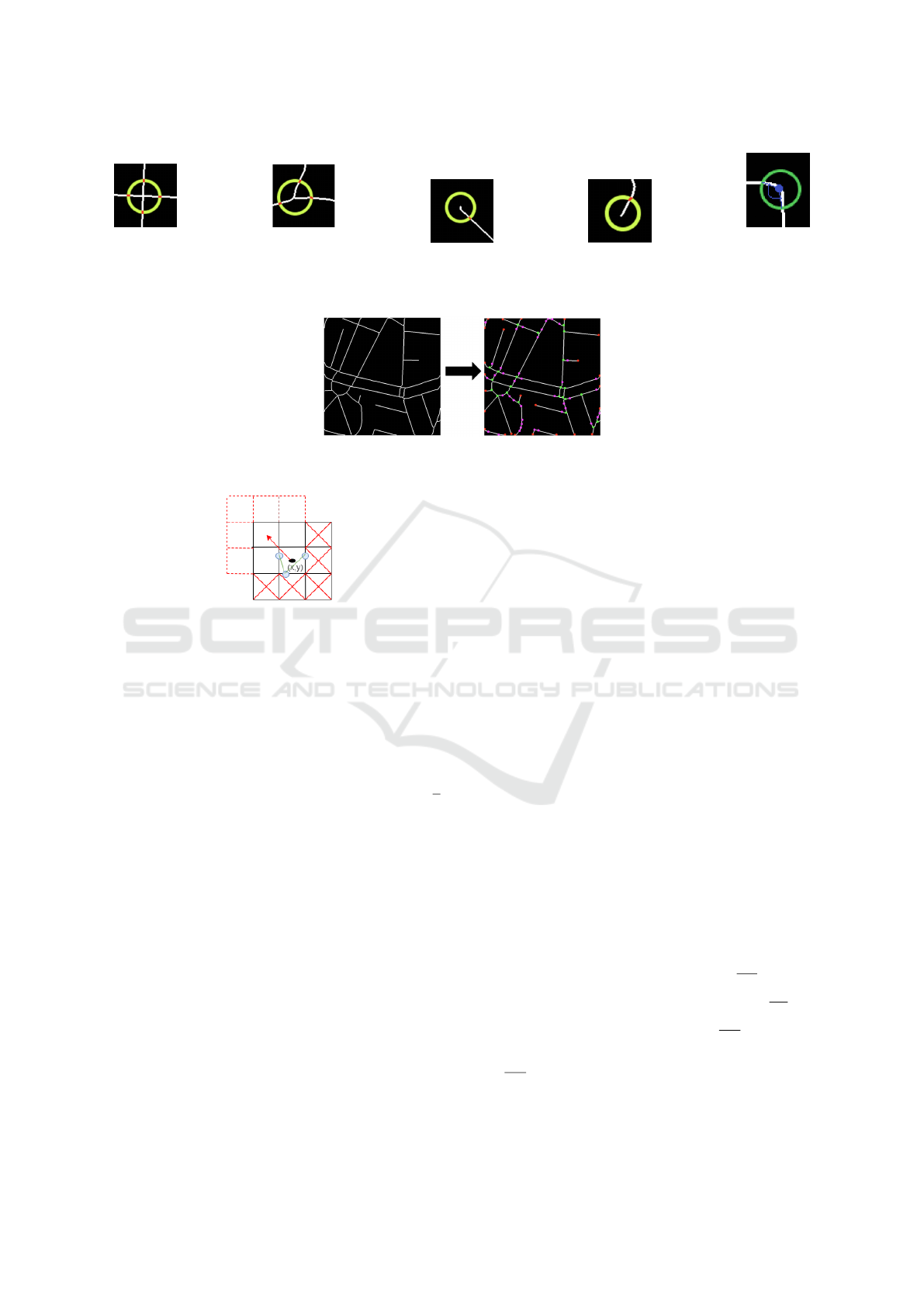
We apply a heuristic to detect the nodes (vertices) of

the graph G describing the roads in the scene. The

heuristic was built as needed on top of the ideas de-

ﬁned in (Mena and Malpica, 2005) to ﬁx some issues

with previous approaches and our dataset. We assume

that the nodes should be located at the elements of

interest: intersections, road ends, and turning points.

For this purpose, we take each white point P in the

given input image (representing a road) and draw a

centered circle in P with radius R (empirically, the

value was set to 5 pixels). If the number of intersect-

ing points (from different road segments) is at least

3, we mark P as an intersection point (Figure 1a, 1b).

If only a single point is intersected, it means that P

is an endpoint of the road (Figure 1c, 1d). To detect

nodes that are turning points, we require that a pair of

distinct nodes in the set of circle intersections form a

turning point of less than TA degrees (empirically, we

chose this value to 90 degrees), Figure 1e. Finally, we

discard points in G that are physically closer than T D

pixels in the input image (chosen as 30 pixels). The

pseudocode of these operations is shown in Listing 1,

while a visualization of a complete example is shown

in Figure 2.

To detect the edges of the graph, a Breadth-First

Search (BFS) is used starting from each node and fol-

lowing the white pixels in the image. Since the road

is larger than one pixel, it is possible to go beyond a

node when searching for connections. To avoid this,

we deﬁne a zone of inﬂuence R for a node so that the

search for a connection node stops when it is in this

area.

At this point, the graph constructed in G has the

network of nodes and road links between them. How-

ever, in order to learn efﬁciently from the data, we

needed some other features that are stored internally:

• The distances between nodes, D(V

, V

• The angles of pairs of nodes representing turning

points, Angle (V

, V

• How many branches each intersection node has,

Inter(V

4 METHODS

Having a dataset of examples in a graph format like

the one described in Section 3, the goal is to continu-

ously generate similar graphs that adhere to the given

patterns and some constraints. In a computer game or

simulation environment, the environment is assumed

to be rendered at a given location (X, Y ). We assume

that the environment can be split into a grid structure

(Figure 3), the rendering effects appear on the current

tile (by default of size 1km in our environment) and

the other 8 tiles in the neighborhood, and each time

the visibility is moved to another tile, a new network

of roads must be generated for the new visible tiles,

while the older tiles that are no longer visible can be

destroyed.

As for the generation process for a single tile, intu-

itively, if one wants to generate a road network simi-

lar to the streets of Manhattan (New York), the streets

should be created primarily in a grid pattern, rather

than the streets of Paris, which have other patterns.

This intuition gave us the idea that the sample graphs

in the database could be grouped into clusters rep-

resenting different levels of granularity (e.g., cities,

neighbourhoods, etc.). A generative model could then

learn the patterns of each cluster and later be used to

create similar looking road networks. Formally, we

divide the database into NK clusters. In the continua-

tion of this section, we describe the clustering and the

two proposed methods for learning generative models

for road networks.

4.1 Clusterization Process

To statistically store the information from each graph

G, and considering that the size of a single physical

example is 512 ×512 pixels, we create the following

measures in order:

Continuous Procedural Network of Roads Generation using L-Systems and Reinforcement Learning

427

(a) Inter-

section

example.

(b) Inter-

section

example.

end point.

(d) Road

end point.

(e) Turn

point

nodes.

Figure 1: Examples of applying the heuristic to ﬁnd different types of nodes in the roads graph.

Figure 2: An example of node detection in a processed image. The nodes at intersections are marked with green color, the

nodes at road ends are marked with red color and the nodes at road turning points are marked with magenta color.

Figure 3: The environment is divided into rectangular tiles

of equal size. If you change the position of the visualiza-

tion from one tile to another, as indicated by the red arrow,

new tiles - the dotted red ones - must be generated, while

unneeded tiles - the ones crossed in red - can be deleted

to save computational resources. The green lines represent

a possible road network within the current tile. The blue

points located at the intersection between the roads within

the tile and the boundary represent the boundary set B of

the current tile.

1. Group the distances between the nodes into 10

equal bins that are between 10 −512 ×512 ×

√

We further denote this as the set G

, i.e. G

[k]

indicates how many distances exist in the group k

in the graph.

2. Group angles representing turning points in 10

equal bins between 0-180. We refer to this as

the set G

, i.e. G

[k] indicates how many turn-

ing points with an angle in group k exist in the

graph.

3. Aggregate the different numbers of branches be-

tween 1 and 10 and group them in the set G

i.e. G

[k] indicates how many intersections with k

branches exist in the given graph.

4. Count the number of intersection nodes, G

, the

total number of end roads, G

, the number of

nodes that are turning points, G

, and the num-

ber of nodes that connect only straight nodes,

. The sum of all interesting nodes in G is then

= G

∔ G

The next step is to use the KMeans (Hartigan and

Wong, 1979) algorithm to group the graphs into K

(user-speciﬁed) groups. In practice, we have con-

cluded that it is best to apply clustering to graphs

that are from the same city. Attempting to cluster

Chicago and Paris, for example, would result in an

interpolation of sparse input data that ultimately does

not represent either city. Instead, it is better for re-

sults to apply the clustering mechanism to each city

individually and then consider different clusters as

parts of the city. The use of standard statistical meth-

ods such as deviations computations are required in

practice to ensure that the data being aggregated and

clustered have the desired input structure. As a sim-

ilarity metric between two graphs G

and G

, we

used the absolute difference between each pair of fea-

tures described in the four metric categories above.

The statistics for the graphs that are part of a clus-

ter K are then aggregated by summing the values for

, G

(we continue to de-

note the aggregations per cluster by K

type

instead of

type

). The following measures and operations are

additionally added for each cluster K to be used later

in the generation process:

• Probability of a turning point: P

• Probability of an intersection point: P

• Probability of an endpoint: P

• Probability of a straight road continuation: P

• A distribution probability for each of the sets K

, K

, representing the distribution of values for

ICSOFT 2022 - 17th International Conference on Software Technologies

428

Listing 1: Pseudocode for adding the road network nodes inside the graph G.

G = {}

f o r e ach wh i t e p i x e l P ( x , y ) :

Draw a c i r c l e of r a d i u s R i n c e n t e r e d i n P

S = s e t o f p o i n t s ( fr om d i s t i n c t s e g m e n t s ) i n t e r s e c t e d by t h e c i r c l e

i f | S | >= 3 : # i n t e r s e c t i o n c a s e

S e t P as i n t e r s e c t i o n no de

G = G U {P }

e l i f | S | == 1 : # r o a d e n d p o i n t c a s e

S e t P as r o a d e n d p o i n t

G = G U {P }

# d e t e c t t u r n i n g p o i n t s

f o r e ac h d i s t i n c t p a i r P1 , P2 o f p o i n t s i n S :

i f a n g l e ( ( P1 − P ) , ( P2 − P ) ) < TA:

S e t P1 and P2 as t u r n i n g p o i n t s

G = G U {P }

E l i m i n a t e n o d e s from G c l o s e r t h a n TD d i s t a n c e from e a c h o t h e r

the set of straight road distances between nodes,

the number of intersections, and the turning an-

gles. A Gaussian mixture model (Reynolds, 2009)

with a number of 3 components (empirically cho-

sen after plotting values from the dataset) is used

and trained using Expectation-Maximization al-

gorithm (Heskes et al., 2004). We further de-

note a sampling process from these as opera-

tions: SampleDist(K), SampleNumBranches(K),

and SampleTurnAngle(K), respectively.

4.2 Generating a Network of Roads for

a Single Tile

At each time the position of the visualization is moved

between tiles, new tiles must be generated as shown in

Figure 3. The proposed process of generating a road

network for a single tile at position (X , Y ) involve the

following steps:

1. If the boundary set of points of the tile, B ̸=

(see below for more details on its construction),

then choose a starting position (x, y) ∈ B.

Otherwise, start from a random position (x, y) in-

side the tile.

2. Set as initial road draw direction the vector from

(x, y) to the center of the tile.

3. Select (manually or randomly) a cluster K to serve

as the representative data sample for the tile.

4. Apply one of the methods deﬁned in Section 4.3

or Section 4.4.

4.3 Generative Model using

Lindenmayer Systems

Parametric and likelihood-based variants of Linder-

mayer Systems (L-Systems ) are used for the ﬁrst gen-

erative model that can generate road networks. For

better understanding of this section, we brieﬂy de-

scribe how L-systems are used in our speciﬁcation.

More details for the interested reader about these sys-

tems and variants can be found in (Rozenberg and Sa-

lomaa, 1980), (Curry, 2000). The L-systems used in

our case consist of a start symbol, a set of rules, and a

set of end conditions. Each rule can optionally spec-

ify a probability for its application, and each symbol

(module) that is modiﬁed can have a set of parame-

ters. A concrete example: A (x, y) : P →A (h, z) means

that the rule is applied to a symbol (module) A with

initial parameters x and y, has a probability P of being

applied, and when applied, changes the values of the

two parameters to h and z, respectively.

In the following, we give the rules for building an

L-system using the statistical data deﬁned in Section

4.1. The system is capable of drawing a complete

road network within a tile starting from given starting

points.

• Start symbol: X .

• Parameters: X (x, y, dir) , where (x, y) is the cur-

rent 2D coordinate in the tile to continue drawing

the road network. The initial position can be cho-

sen randomly or can start from the boundary of a

neighbouring tile (the set B deﬁned below in the

stop condition). The current drawing direction is

Continuous Procedural Network of Roads Generation using L-Systems and Reinforcement Learning

429

parameterized by d, which is a 2D vector. The

number of operations on the same path is stored

internally in a variable age (not shown in the rules

below for simplicity), which is mainly used to

stop the process when possible inﬁnite loops are

detected.

• Rules: Draw a sample from a uniform random

variable (0-1), then decide which item to generate

next based on the probabilities and using a roulette

wheel, in the following order:

– Draw a straight connection from a previous

point and keep the same direction:

X (x, y, d) : P

→ X ((x, y) ∔ d ×r, d)

, wherer = S ampleDist (K)

– Change the current direction with a new sam-

pled direction:

X (x, y, d) : P

→ X (x, y, newDir)

, wherenewDir = SampleTurnAngle (K)

– Create a road end:

X (x, y, d) : P

→ E (x, y)

, wherenewDir = SampleTurnAngle (K)

– At an end of road symbol we stop the process:

E (x, y) →

– Create an intersection with a sampled number

of branches and split the drawing process into

several parallel directions:

X (x , y, d) : P

→ X (x, y, nd

)|...|X (x, y, nd

)

, wherenB = SampleNumBranches(K)

, and nd

= SampleTurnAngle(K) withi ∈ 1 . . . nB

• Condition for a hard stop: the coordinate param-

eters (x, y) are outside the speciﬁed tile. In this

case, the algorithm stores the intersection point

between the previous coordinate set and (x, y) as

a boundary point and adds it to a group of points

At each step deﬁned above, the new position (x, y)

is added as a new node to the generated graph, with

the appropriate label and with an edge connecting the

previously generated point. To ensure the quality of

the results, we do not allow self-intersection during

generation, i.e., we rerun the sample if the new posi-

tion would lead to self-intersection.

4.4 Model using Reinforcement

Learning

For this task, we have currently chosen the Double

Q-Learning (DDQN) method (Hasselt, 2010).

The set of actions that the agent can perform at

each step is similar to our previous approach with

Lindenmayer Systems. At each step, the agent must

choose between creating a straight road segment of a

certain length, changing the drawing angle by a cer-

tain number of degrees, creating an intersection with

a certain number of branches, or creating an end of

road. The actions are thus encoded in this order with

indices between 0 −3. The speciﬁc values to be ap-

plied are sampled from the learned data distribution

as before.

The state of the environment seen by the agent at

each step is deﬁned by a state composed of 10 input

parameters: the number of nodes of each type, the

length of the last segment, the direction of the current

drawing direction, the current and previous drawing

positions, the branches of the last intersection, and

the last action performed. These inputs are passed

through two fully connected neural layers with 32 and

8 neurons, respectively for further processed.

We do not explicitly describe the details of the

reward function, but instead explain the rules used

to achieve good RL agent results with the algorithm

used:

• We encourage segments of average value in the

detriment of very long or short segments.

• We gradually penalize very close angles (e.g., less

than 30 degrees).

• We penalize new segments if they go out of

bounds or self-intersect the existing road.

• We encourage road ends a little less than other el-

ements, so that the road does not end so quickly.

• We encourage the creation of a new segment after

a change in direction.

• We encourage the creation of a direction change

after a new intersection.

• We penalize the creation of a similar element in a

row.

Future work will also investigate whether the pol-

icy gradient class algorithms (Sutton and Barto, 2018)

could provide better results in certain cases. In ad-

dition, further research needs to evaluate whether

adding the image drawn at each time point can be ef-

ﬁciently used as input by convolutional layers. The

results of our current evaluation are inconclusive in

these cases.

5 EVALUATION

As mentioned in the Section 2, there was no similar

work in terms of requirements, i.e., mimicking the

ICSOFT 2022 - 17th International Conference on Software Technologies

430

real world or given user input with real-time usage)

that could be compared to our presented work. In-

stead, in the following text, we make an evaluation of

the proposed generative methods from different per-

spectives.

5.1 Qualitative Results Comparison

It is difﬁcult to visually compare the results between

the L-systems and the RL-based systems. However,

from our observation, the RL-based method has a dif-

ferent degree of sampling for stochastic variables in

theory, which translates into a more diverse road net-

work in practice. However, the advantage of using

L-systems, is that the user can constrain and con-

trol the generation process in deeper details, which

could be an important decision in some ﬁelds, such as

game development. To test whether the patterns of a

given city can be reproduced and the models indeed

generate similar content, we selected a subset of two

cities, Paris (city center) and Chicago, from the orig-

inal dataset and applied our method to test whether

the inference leads to similar results. This overﬁtting

test showed that both low-level methods can produce

similar content to the original data without signiﬁ-

cant visual differences, while still showing the orig-

inal roads patterns. However, for both methods, we

constrained the environment and methods to produce

self-overlapping results. Without this hard constraint,

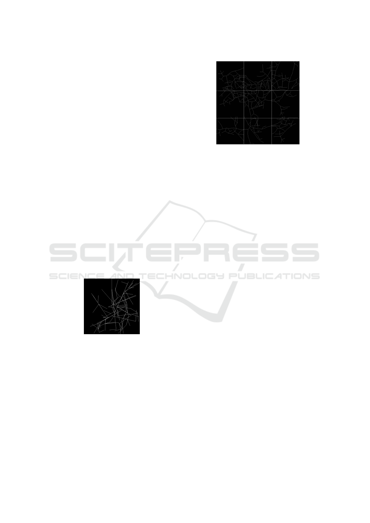
we obtain results similar to those in Figure 4.

Figure 4: A typical result that might occur if you do not use

the self-intersecting hard constraint.

Figure 5 shows a ﬁnal result for creating a 3 ×3

grid structure from a portion of the Paris city map.

Note also that our generation process can work

with inputs learned from user-deﬁned datasets, re-

gardless of the patterns they exhibit. Following the

tile selection cluster method we introduced in Section

4.1, the user can switch patterns for individual clus-

ters at runtime. In a computer game, for example, this

can be used to switch between different parts of the

worlds or to create custom mini-games. One limita-

tion of our method is that we do not learn anything

about the elevation of the ground at this point. This

has been left as future work.

Figure 5: Network of roads on a 3 ×3 tiled environment

generated using our methods based on a some speciﬁc part

of Paris city map.

5.2 Runtime Performance

To ﬁnd out if the method is suitable for real-time

evaluation, we compared the generation of a different

number of tiles at once (1 to 9) with both methods on

an Intel Core i7 11700k CPU. Since nowadays paral-

lelism is also heavily used in games or simulation en-

gines, we evaluated both sequential and parallel com-

puting time considering 8 worker threads, each as-

signed to a different CPU core (i.e., a parallel task for

each tile). The results shown in Table 1 indicate that

the method is suitable for real-time use, even when

the visualization perspective is heavily modiﬁed, i.e.

when many tiles need to be generated at once. Us-

ing L-Systems as the base method provides a slight

advantage, at the cost of a possible lower variety of

generated environments as noted above.

6 CONCLUSION AND FUTURE

WORK

This paper presented ﬁrst methods for generating a

continuous road network in large environments that

mimics the patterns of real-world cities. The evalu-

ation section has shown that our proposed methods

are generally suitable for use at runtime in applica-

tions such as computer games or simulation environ-

ments. Second, we presented a set of scripts that can

transform a dataset of top-down pictures of real-world

cities into graph augumented structures that the com-

munity can experiment with further, and made them

available as open source. We plan to continue our

work on procedural content generation, particularly in

creating models capable of generating content around

these roads. Possible examples could include vegeta-

tion, buildings, etc. We are also looking forward to

expanding the augmented data structures used and in-

Continuous Procedural Network of Roads Generation using L-Systems and Reinforcement Learning

431

Table 1: Comparative runtime evaluation (milliseconds) between methods using reinforcement learning, L-Systems, both

sequential and parallel with 8 worker threads.

Number of tiles 1 2 3 4 5 6 7 8 9

Sequential RL 2.03 4.43 7.88 10.4 12.81 15.79 18.21 21.41 23.42

Parallel RL 2.14 3.61 6.33 8.21 9.89 11.83 12.98 13.99 14.61

Sequential LS 1.76 3.98 7.72 10.29 10.63 13.73 18.02 20.33 22.48

Parallel LS 1.99 2.92 5.12 7.71 8.60 11.59 12.33 13.29 14.46

clude terrain elevation. In terms of methodology, we

plan to explore other methods for generating similar

or combined content.

REFERENCES

Bojchevski, A., Shchur, O., Z

ugner, D., and G

unnemann, S.

(2018). Netgan: Generating graphs via random walks.

Chen, G., Esch, G., Wonka, P., Mueller, P., and Zhang, E.

(2008). Interactive procedural street modeling. ACM

Trans. Graph., 27(3):Article 103: 1–10.

Curry, R. (2000). On the evolution of parametric l-systems.

Danny Alberto, E. C., Luo, X., Navarro Newball, A. A.,

niga, C., and Lozano-Garz

on, C. (2019). Realis-

tic behavior of virtual citizens through procedural an-

imation. In 2019 International Conference on Virtual

Reality and Visualization (ICVRV), pages 243–247.

de Ara

ujo, L. J. P., Grichshenko, A., Pinheiro, R. L.,

Saraiva, R. D., and Gimaeva, S. (2020). Map gen-

eration and balance in the terra mystica board game

using particle swarm and local search. In Tan, Y., Shi,

Y., and Tuba, M., editors, Advances in Swarm Intelli-

gence, pages 163–175, Cham. Springer International

Publishing.

Dong, J., Liu, J., Yao, K., Chantler, M., Qi, L., Yu, H., and

Jian, M. (2020). Survey of procedural methods for

two-dimensional texture generation. Sensors, 20(4).

Freiknecht, J. and Effelsberg, W. (2017). A survey on the

procedural generation of virtual worlds. Multimodal

Technologies and Interaction, 1(4).

Gissl

en, L., Eakins, A., Gordillo, C., Bergdahl, J., and Toll-

mar, K. (2021). Adversarial reinforcement learning

for procedural content generation.

Hartigan, J. A. and Wong, M. A. (1979). A k-means cluster-

ing algorithm. JSTOR: Applied Statistics, 28(1):100–

108.

Hasselt, H. (2010). Double q-learning. In Lafferty, J.,

Williams, C., Shawe-Taylor, J., Zemel, R., and Cu-

lotta, A., editors, Advances in Neural Information

Processing Systems, volume 23. Curran Associates,

Inc.

Heskes, T., Zoeter, O., and Wiegerinck, W. (2004). Approx-

imate expectation maximization. In Thrun, S., Saul,

L., and Sch

olkopf, B., editors, Advances in Neural In-

formation Processing Systems, volume 16. MIT Press.

Kipf, T. N. and Welling, M. (2016). Variational graph auto-

encoders.

Lara-Cabrera, R., Cotta, C., and Fern

andez-Leiva, A.

(2012). Procedural map generation for a rts game.

Li, Z., Wegner, J. D., and Lucchi, A. (2019). Topological

map extraction from overhead images. In Proceedings

of the IEEE/CVF International Conference on Com-

puter Vision (ICCV).

Liu, J., Snodgrass, S., Khalifa, A., Risi, S., Yannakakis,

G. N., and Togelius, J. (2020). Deep learning for pro-

cedural content generation. Neural Computing and

Applications, 33(1):19–37.

Mena, J. and Malpica, J. (2005). An automatic method for

road extraction in rural and semi-urban areas starting

from high resolution satellite imagery. Pattern Recog-

nition Letters, 26(9):1201–1220.

Parish, Y. I. H. and M

uller, P. (2001). Procedural model-

ing of cities. In Proceedings of the 28th Annual Con-

ference on Computer Graphics and Interactive Tech-

niques, SIGGRAPH ’01, page 301–308, New York,

NY, USA. Association for Computing Machinery.

Ping, K. and Dingli, L. (2020). Conditional convolutional

generative adversarial networks based interactive pro-

cedural game map generation. In Arai, K., Kapoor,

S., and Bhatia, R., editors, Advances in Information

and Communication, pages 400–419, Cham. Springer

International Publishing.

Reynolds, D. (2009). Gaussian Mixture Models, pages 659–

663. Springer US, Boston, MA.

Rozenberg, G. and Salomaa, A. (1980). Mathematical The-

ory of L Systems. Academic Press, Inc., USA.

Snodgrass, S. and Onta

on, S. (2017). Learning to gen-

erate video game maps using markov models. IEEE

Transactions on Computational Intelligence and AI in

Games, 9(4):410–422.

Sutton, R. S. and Barto, A. G. (2018). Reinforcement Learn-

ing: An Introduction. A Bradford Book, Cambridge,

MA, USA.

Wang, H., Wang, J., Wang, J., Zhao, M., Zhang, W.,

Zhang, F., Xie, X., and Guo, M. (2017). Graphgan:

Graph representation learning with generative adver-

sarial nets.

Zhou, D., Zheng, L., Xu, J., and He, J. (2019). Misc-gan:

A multi-scale generative model for graphs. Frontiers

in Big Data, 2:3.

ICSOFT 2022 - 17th International Conference on Software Technologies

432