A Comparison of Automatic Labelling Approaches for Sentiment

Analysis

Sumana Biswas, Karen Young and Josephine Grifﬁth

School of Computer Science, National University of Ireland, Galway, Ireland

Keywords:

Sentiment Analysis, NLP, Deep Learning, Automatic Labelling.

Abstract:

Labelling a large quantity of social media data for the task of supervised machine learning is not only time-

consuming but also difﬁcult and expensive. On the other hand, the accuracy of supervised machine learning

models is strongly related to the quality of the labelled data on which they train, and automatic sentiment

labelling techniques could reduce the time and cost of human labelling. We have compared three automatic

sentiment labelling techniques: TextBlob, Vader, and Aﬁnn to assign sentiments to tweets without any human

assistance. We compare three scenarios: one uses training and testing datasets with existing ground truth

labels; the second experiment uses automatic labels as training and testing datasets; and the third experiment

uses three automatic labelling techniques to label the training dataset and uses the ground truth labels for

testing. The experiments were evaluated on two Twitter datasets: SemEval-2013 (DS-1) and SemEval-2016

(DS-2). Results show that the Aﬁnn labelling technique obtains the highest accuracy of 80.17% (DS-1) and

80.05% (DS-2) using a BiLSTM deep learning model. These ﬁndings imply that automatic text labelling could

provide signiﬁcant beneﬁts, and suggest a feasible alternative to the time and cost of human labelling efforts.

1 INTRODUCTION

Social media facilitates the sharing of ideas, views,

and emotional responses between people. In these

interactions, people often use short-text, meaningless

unofﬁcial words, short words, and emoticons, which

can make it confusing to understand the exact mean-

ing of the text. Sentiment analysis can be deﬁned as a

technique for classifying emotions into binary (Posi-

tive, and Negative) or ternary (Positive, Negative, and

Neutral) classes. Extracting sentiment from this typ-

ically unstructured social media data is challenging

and presents a difﬁcult problem for researchers in this

space. Analysing opinions is important because it can

provide useful information for speciﬁc products, per-

spectives, or commentary on world events. Success-

ful sentiment analysis of textual information (Daniel

et al., 2017; Xu et al., 2019) depends on three main

elements: a meaningful and clear expression of con-

text; correctly labelled training and test datasets; and

a suitable machine learning algorithm capable of ac-

curately characterizing sentiment.

The labelling of social media data is an open

problem for researchers when analysing sentiment.

Although, it is easy and cheap to get labelled data

from some online crowdsourcing systems like Rent-

A-Coder, Amazon Mechanical Turk, etc. (Snow et al.,

2008; Whitehill et al., 2009), in many cases, one has

no idea about the availability, efﬁciency, and quality

of the labellers for a speciﬁc ﬁeld or task. Labelling

errors from non-expert labellers, and biased labelling

due to a lack of efﬁciency, can result in incorrect and

imbalanced labelling. The alternative, to ensure high-

quality labels, is to engage human experts to perform

the labelling, but this is both time-consuming and ex-

pensive. However, comparisons have not been car-

ried out on evaluating the difference in performance

of machine learning models when using automatic

versus human labelling. There has been very little

study done to support or recommend the best labelling

method. The lack of evaluation of these automatic la-

belling approaches motivates our work.

In this study, we have compared three state-of-

the-art automatic labelling methods with the inten-

tion of quickly producing sentiment labels for Twit-

ter data without human involvement. We have eval-

uated our approaches on two larger datasets from

the SemEval-13 and SemEval-16 competitions, which

contain ground truth and act as our human labelling.

In this paper, we will use the term ‘Human La-

belling’(HL) as ground truth throughout the discus-

sion. The labels: ‘Positive’, ‘Negative’, and ‘Neutral’

312

Biswas, S., Young, K. and Grifﬁth, J.

A Comparison of Automatic Labelling Approaches for Sentiment Analysis.

DOI: 10.5220/0011265900003269

In Proceedings of the 11th International Conference on Data Science, Technology and Applications (DATA 2022), pages 312-319

ISBN: 978-989-758-583-8; ISSN: 2184-285X

are classiﬁed and assigned by the analysis of word

meanings and polarity scores according to the word

features and patterns. Three lexicon-based state-

of-the-art automatic labelling approaches: TextBlob,

Aﬁnn, and Vader are used to generate all sentiment la-

bels. The results of automatic labelling are compared

to the results of human labelling using deep learning

algorithms for sentiment analysis in order to deter-

mine reasonable alternatives to labelling social media

data. The main objectives of our work are as follows:

• Assign sentiment labels to the Twitter datasets

using three automatic labelling methods: Aﬁnn,

TextBlob, and Vader.

• To establish whether automatic labelling ap-

proaches would be a viable alternative as com-

pared with human labelling in terms of reducing

the time and expense of human labelling.

• To obtain the best deep learning algorithm to anal-

yse sentiment when the Twitter datasets are la-

belled by three automatic labelling approaches.

The paper is organized as follows: in Section 2, re-

lated work on labelling strategies for state-of-the-art

classiﬁer methods and sentiment analysis approaches

is presented. Section 3 describes our methodology,

while Section 4 details the experiment and discusses

the results. Finally, Section 5 concludes the paper

with a discussion of limitations and plans for future

work.

2 RELATED WORK

Sentiment analysis is a challenging problem due to

the features of natural languages, such as the use

of words in different situations, indicating different

meanings. Sentiment analysis approaches are evalu-

ated on datasets with either human labels (Moham-

mad et al., 2016; Mohammad et al., 2017; Deriu

et al., 2016) or automatic labels (Saad et al., 2021;

Chakraborty et al., 2020). Human annotators assign

the sentiment labels for training and testing datasets

by their understanding and expertise. Most of the

datasets are annotated by human experts for rela-

tively small datasets. For example, (Deriu et al.,

2016; Mohammad et al., 2016) used human labelling

to predict sentiment. But, Oberlander and Klinger

(2018) found noisy labels (Sheng et al., 2008) in

the largest human annotated dataset (39k) (Crowd-

Flower, 2016). Several authors (Dimitrakakis and

Savu-Krohn, 2008; Lindstrom et al., 2010; Turney,

1994) studied data labelling costs and found that ob-

taining high-quality labelled data is time-consuming

and cost-ineffective. The alternative of obtaining sen-

timent labels using automatic labelling saves time and

money. The lexicon-based automatic labelling tech-

niques of TextBlob, Vader, and Aﬁnn use the NLTK

(Natural Language Toolkit) of python libraries to au-

tomatically classify the sentiment of text and have

been used in many studies. Each lexicon-based sen-

timent labelling approach needs a predeﬁned word

dictionary to infer the polarity of the sentiment ac-

cording to their rules. Vader dictionaries are used to

ﬁnd the polarity scores of each word. Deepa et al.

(2019) assessed the polarity scores of words to cate-

gorize the sentiment for the Twitter dataset related to

UL Airlines with human labels using two dictionary-

based methods: Vader dictionaries and Sentibank;

the Vader dictionaries outperformed Sentibank by 3%

in their analysis to detect the polarity scores for the

sentiment classiﬁcation using the Logistic Regres-

sion (LR) model. TextBlob and Aﬁnn were used by

(Chakraborty et al., 2020) to label a large number

of tweets (226k) using ternary classes. They found

that TextBlob labelling generated normalized scales

of the sentiment labels compared to the Aﬁnn la-

belling and obtained 81% accuracy in the LR clas-

siﬁcation method. Then, they proposed a fuzzy in-

ference rule that used the Vader dictionaries to as-

sign ternary sentiment labels and got 79% accuracy

in predicting the sentiment of sentences using the

Gaussian membership function. Saad et al. (2021)

used Aﬁnn, TextBlob, and Vader to assign sentiment

labels to a drug review dataset, and they obtained

96% accuracy with TextBlob; similarly, (Hasan et al.,

2018) and (Wadera et al., 2020) also got success with

TextBlob labelling on Twitter datasets using some of

the traditional machine learning algorithms like Sup-

port Vector Machine (SVM), Na

ıve Bayes (NB), Ran-

dom Forest Tree (RFT), Decision Trees (DTC), and

K-Nearest Neighbours (KNN). There is no one auto-

matic labelling technique that does best consistently

in the previous work, and all the evaluations used ei-

ther human labelling or automatic labelling, but they

did not use both labelling strategies and did not com-

pare them.

State-of-art deep learning algorithms have been

used to predict the sentiment of text that is shared on

different social media in several studies (Poria et al.,

2015; Lei et al., 2016). Liao et al. (2017) proposed

a one-layer Convolution Neural Network (CNN) to

analyse the sentiment. Similarly, Long Short Term

Memory (LSTM), Bidirectional (BiLSTM) models

are also used in natural language processing (Xu et al.,

2019). However, all the above research used human

labelling in their state-of-the-art deep learning algo-

rithms, but they did not use automatic labelling.

A Comparison of Automatic Labelling Approaches for Sentiment Analysis

313

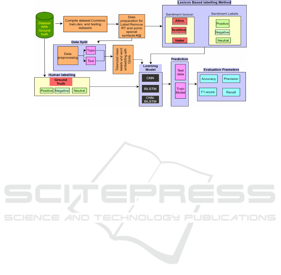
Figure 1: A summary of the experiments performed.

3 METHODOLOGY

We have used two Twitter datasets from the SemEval-

13 and SemEval-16 competition which contains hu-

man labels (HL). We did not consider the remaining

datasets from this competition because they had ei-

ther imbalanced human labels or had a small number

of tweets. The details of the datasets are given in the

paper (Deriu et al., 2016) and (Yoon and Kim, 2017).

SemEval-2013 Task 4 and SemEval-2016 Task-4 are

named as DS-1 and DS-2 respectively in this study.

The original datasets are divided into train, dev, and

test. We combine the training, development, and test-

ing portions of each dataset to create a single whole

dataset. The ﬁrst experiment uses the existing Se-

mEval labels (human labels) for both training and

testing. The second experiment uses, in turn, the

three automatic labelling methods (TextBlob, Vader,

and Aﬁnn) for both the training and testing datasets.

The third experiment uses the existing SemEval labels

(human labels) for testing, but the training data labels

are generated using, in turn, the three automatic la-

belling methods (TextBlob, Vader, and Aﬁnn). In all

cases, 80% of each dataset is used for training and the

remaining 20% of the dataset is used for testing. For

each experiment, CNN, BiSLTM, and CNN-BiSLTM

deep learning algorithms are applied to the cleaned

and pre-processed training data and the models are

tested on the test data. Figure 1 illustrates the details

of the methodology which is explained in the follow-

ing steps.

3.1 Data Labelling

In experiment 2 for both training and testing datasets

and in experiment 3 for only the training dataset, we

replace the human labels with automatically gener-

ated labels. Prior to assigning the automatic labels,

we remove the username and some special symbols

such as @, #, $, and RT from all tweets in the datasets.

We have used the Natural Language Toolkit (NLTK)

library from Python to label the tweet’s sentiment

as Positive, Negative or Neutral using the following

three methods:

TextBlob: In this study, we have used the polarity

of sentiment for textual data among the many proper-

ties available as part of TextBlob in the Python library.

TextBlob returns a polarity value within the range [-

1.0, 1.0] where ‘-1’ indicates a very Negative polarity,

‘0’ a Neutral polarity and ‘+1’ is a very Positive po-

larity.

Vader: VADER stands for ‘Valence Aware Dic-

tionary and sEntiment Reasoner’ (Hutto and Gilbert,

2014). It is a rule-based sentiment analysis tool,

which generates the scores of sentiments by the in-

tensity of lexical features and semantic meanings of

the text. Vader returns four components with associ-

ated intensity scores. For example, {neg: 0.106, neu:

0.769, pos: 0.125, compound: 0.1027}, where ‘neg’,

‘neu’, ‘pos’ indicate the Negative, Neutral, and Pos-

itive scores respectively and the compound score is

the normalized score of the summation of the valence

scores computed based on heuristic and lexicon senti-

ments. In this study, we assign ‘Positive’ label when

the compound score is greater than 0.05, ‘Negative’

label when the compound score is less than -0.05 and

otherwise, we assign ‘Neutral’ label.

Aﬁnn: Aﬁnn is a simple and popular lexicon de-

veloped by Finn Arup Nielsen (Nielsen, 2011). Aﬁnn

returns the score of a word between [-5, 5]. Here we

assign a ‘Positive’ label when the score is greater than

‘0’, a ‘Negative’ label when the score is less than ‘0’

DATA 2022 - 11th International Conference on Data Science, Technology and Applications

314

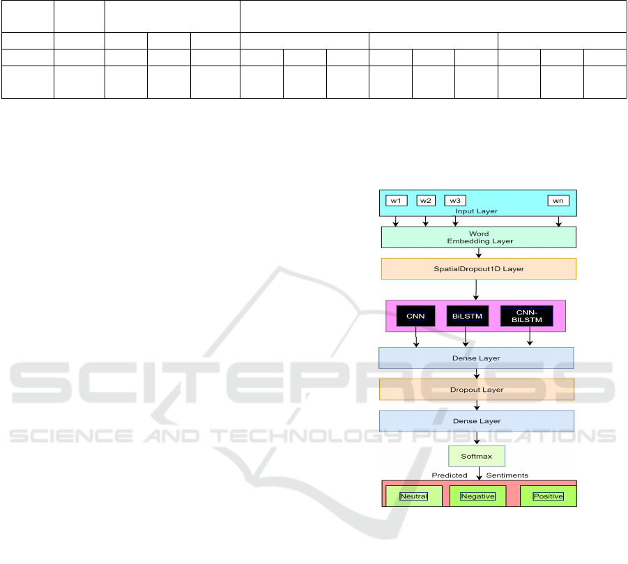
Table 1: Summary statistics of the total number of tweets from the SemEval competitions Tweet-2013 (DS-1) and Tweet-2016

(DS-2), and the percentage of Positive (Pos.), Negative (Neg.), and Neutral (Neut.) sentiment labels from human labelling

and automatic labelling approaches (TextBlob, Vader, Aﬁnn).

Dataset Total

Tweets

Human Labelling(%) Automatic Labelling(%)

TextBlob Vader Aﬁnn

Pos Neg Neut Pos Neg Neut Pos Neg Neut Pos Neg Neut

DS-1 14885 38.23 15.84 45.94 48.66 19.55 31.41 51.55 18.2 29.99 45.76 17.96 36.01

DS-2 28631 38.41 15.67 45.93 46.34 20.28 32.4 47.06 24.48 27.48 42.1 22.87 34.05

and otherwise we assign a ‘Neutral’ label.

To illustrate the automatic labelling techniques we

take as an example from DS-2: “install the newest

version and you may change your mind!”; the sen-

timent label is assigned as ‘Neutral’, ‘Positive’, and

‘Positive’ using the TextBlob, Vader and Aﬁnn meth-

ods respectively. It is noted that the existing human

(ground truth) label of the same text is also ‘Positive’.

Table 1 presents the two datasets with the original

name, the newly assigned name in our experiments,

and the total number of tweets associated with each

dataset. It also shows the summary of the percent-

age of sentiment labels per dataset with the automatic

labelling approaches in comparison to the human la-

bels. Positive labels are remarkably high when using

automatic labelling techniques. On the other hand,

Neutral labels are notably high in the human labelled

datasets.

3.2 Data Preprocessing for Models

Data pre-processing and cleaning is an important step

when applying deep learning algorithms to the data.

We remove any unwanted words using a list of stop

words from the NLTK (Natural Language Toolkit) li-

brary in Python, without removing stop words like

‘our’, ‘ours’, ‘ourselves’, ‘these’, ‘those’ etc. We

removed all digits in the tweets and some unwanted

words which did not make any sense like ‘amp’, ‘tik-

tok’, ‘th’, etc., and inappropriate words. The cleaned

tweets are then tokenized after being split into train-

ing and testing sets. We have used GloVe of 300 di-

mensions for word embedding. GloVe, which stands

for Global Vectors, is an unsupervised learning algo-

rithm for achieving vector representations of words.

Large quantities of text are used for training and con-

verting into low dimensional and dense word forma-

tions in an unsupervised fashion by an embedding

process (Pennington et al., 2014). One hot encoding

is a highly popular technique to deal with categorical

data, which creates a binary column for each category

and returns a sparse matrix or dense array based on

the sparse parameter. We have labelled the sentiments

of tweets in three categories and used the one-hot en-

coding method. For this, three new columns are cre-

ated as ‘Positive’, ‘Negative’, and ‘Neutral’, and these

dummy variables are then ﬁlled up with Zeros (mean-

ing False) and ones (meaning True).

Figure 2: Structure of the deep learning models.

3.3 Deep Learning Models

This section describes the method of using deep learn-

ing models. CNN (Convolution Neural Network),

BiLSTM (Bidirectional Long Short-Term Memory),

and a combined model of CNN-BiLSTM are used to

ﬁnd the sentiments of tweets. The model consists of

some common layers: an embedded layer, a Spatial-

Dropout1D layer, a deep learning layer, Dense layer,

Relu dense layer, Dense, and ﬁnally a Softmax layer

to predict sentiments. Three deep learning models:

CNN, BiLSTM, and CNN-BiLSTM are used sepa-

rately in the deep learning layer, which is in between

the SpatialDropout1D layer and the Dense layer of

the common layers. The architecture of the mod-

els is shown in Figure 2. A SpatialDropout1D layer

takes a word embedding matrix of an input sentence;

A Comparison of Automatic Labelling Approaches for Sentiment Analysis

315

It helps to prevent pixels from co-adapting with their

neighbors across feature maps, which promotes inde-

pendence between feature maps. The output is fed

to different deep learning networks. Each output of

the three deep learning models is fed separately into a

dense layer with a Relu activation function, and then

a ﬁnal dense layer with a softmax activation function

predicts the probabilities of ternary sentiment labels.

CNN: A CNN is a feed-forward neural network

containing an input layer, hidden layer and an output

layer, which is capable of capturing all local features.

It computes the most important features from the out-

put of the CNN (Liao et al., 2017) with a Rectiﬁed

Linear Unit (ReLU) activation, and Global max pool-

ing layer.

BiLSTM: Long Short-Term Memory (LSTM) is a

Recurrent Neural Network (RNN) with three gates:

input gate, output gate, and forgot gate (Xu et al.,

2019). It has a forward and backward layer. BiLSTM

is capable of remembering future and past informa-

tion from input sequences and processing the infor-

mation in both directions.

CNN-BiLSTM: A CNN model is combined with

a BiLSTM (Xu et al., 2019) model. CNN-BiLSTM

includes all prominent level features and long-term

dependencies in both directions (Chaturvedi et al.,

2018) of input datasets for all labelling strategies in

the aforementioned three experiments.

3.4 Experiment Setup

Each deep learning model takes inputs from the Spa-

tialDropout1D layer which is embedded with se-

quence input. The maximum input sequence length

is 30. The CNN layer uses 64 ﬁlters with kernel

size 5. The BiLSTM layer is used with 64 hidden

units. A fully connected layer also is used with 64

hidden units. To avoid over ﬁtting and under ﬁt-

ting, CNN uses two dropout levels and BiLSTM and

CNN-BiLSTM models employ four dropout levels.

To get good results for different algorithms, we chose

varied drop out rates. For example, in the ﬁrst ex-

periment, the drop out rates in the CNN model are

(0.2 and 0.2), however in the second and third ex-

periments, the drop out rates are (0.4, 0.5) and (0.3,

0.5), respectively. In the ﬁrst, second, and third ex-

periments, the dropout rates for BiLSTM and CNN-

BiLSTM are (0.3,0.3,0.3,0.4), (0.2,0.2,0.2,0.5), and

(0.3,0.3,0.3,0.5), respectively. We have set a learn-

ing rate of 0.0001 for the ﬁrst experiment (human la-

belling). A learning rate of 0.001 is considered for

the second and third experiments. Categorical cross-

entropy is used as the loss function and categorical

accuracy is used for the accuracy metric. We set the

batch size to be 100 and run for 10 epochs to aver-

age the metrics for accuracy, precision, F1 scores and

recall.

4 EXPERIMENT RESULTS AND

DISCUSSION

The performance of the models is measured by us-

ing four possible outcomes: True Positives (TP), True

Negatives (TN), False Positive (FP), and False Nega-

tive (FN). The accuracy of the result is computed us-

ing those outcomes, but accuracy can mislead in im-

balanced datasets. This is why, we have computed

precision, recall, and F1-score. Table 2 shows the re-

sults of the ﬁrst experiment, which used three deep

learning models with human labelling for the two

datasets. The results are evaluated in macro averaged

performance across the Positive, Negative, and Neu-

tral classes. The BiLSTM model obtains the highest

accuracy, precision, F1-score and recall for the two

datasets. The best results are highlighted in bold in

the result Tables. The accuracy of the BiLSTM model

is 1.19% higher than the CNN model and 0.93%

higher than the CNN-BiLSTM model for DS-1. In

the same way, the accuracy of the BiLSTM model is

5.57 and 3.48% higher than the accuracy of the CNN

and CNN-BiLSTM model respectively for DS-2. The

F1-score is also higher with the BiSLTM model than

the other two models.

The results of the second experiment are shown in

Table 3 using the three automatic labelling strategies

and the three deep learning algorithms. The results

show higher accuracy, precision, recall, and F1-scores

for the two datasets with automatic labelling than hu-

man labelling. Additionally, Aﬁnn labelling obtains

the highest accuracy using the BiLSTM model for

the two datasets compared to the other models with

TextBlob and Vader labelling techniques. The bal-

ance of sentiment labels are better in Aﬁnn labelling

than the other labelling techniques, and this could ex-

plain why Aﬁnn does better than the other labelling

strategies. On the other hand, the CNN model could

not learn all the dependencies of whole sentences

due to the limitation of ﬁlter lengths (Camg

ozl

u and

Kutlu, 2020). As a result, CNN and CNN-BiLSTM

models were not able to learn all features from sen-

tences or whole datasets. For this reason, BiLSTM

outperformed the other models with F1 scores of

77.54% and 80.7% for DS-1 and DS-2 respectively.

In the third experiment, we have observed the re-

sults with 80% of the training data with automatic la-

belling and 20% of test data with human labelling.

Table 4 displays the results of the third experiment

DATA 2022 - 11th International Conference on Data Science, Technology and Applications

316

Table 2: Experiment 1: Comparison of Accuracy, Precision, F1-score and Recall with human labels using a CNN, BiLSTM,

and CNN-BiLSTM Model.

Model DS-1(%) DS-2(%)

Acc Pre F1 Rec Acc Pre F1 Rec

CNN+HL 60.36 65.50 55.19 52.08 54.97 66.92 56.39 50.48

BiLSTM+HL 61.55 71.95 58.25 54.25 60.54 66.79 61.99 57.99

CNN-BiLSTM+HL 60.62 63.82 55.97 53.99 57.06 66.14 57.74 52.93

Table 3: Experiment 2: Comparison of Accuracy, Precision, F1-Score and Recall with automatic labelling used for both

testing and training datasets using CNN, BiLSTM, and CNN-BiLSTM Models.

Model DS-1(%) DS-2(%)

Acc Pre F1 Rec Acc Pre F1 Rec

CNN+Af 74.26 76.51 72.24 69.37 74.28 77.48 74.39 71.67

BiLSTM+Af 80.17 81.63 77.54 74.92 80.05 84.06 80.70 77.80

CNN-BiLSTM+Af 75.27 78.11 73.04 69.79 76.9 81.16 77.9 74.93

CNN+Tb 63.17 73.70 61.37 55.60 69.27 76.09 69.69 65.8

BiLSTM+Tb 73.41 77.38 72.06 68.75 79.55 82.67 78.77 76.44

CNN-BiLSTM+Tb 66.95 72.77 65.00 61.15 75.03 78.46 74.5 71.92

CNN+Vd 68.22 72.8 66.17 62.37 68.19 76.09 71.04 67.03

BiLSTM+Vd 73.75 75.99 70.64 68.53 76.79 79.29 76.63 75.0 6

CNN-BiLSTM+Vd 71.12 73.46 66.96 63.81 72.4 76.58 73.56 70.89

Table 4: Experiment 3: Comparison of Accuracy, Precision, F1-score and Recall with automatic labelling techniques (training

dataset) and human labelling for the test set using CNN, BiLSTM, and CNN-BiLSTM Models.

Model DS-1(%) DS-2(%)

Acc Pre F1 Rec Acc Pre F1 Rec

CNN+Af 57.49 60.03 54.91 51.97 46.57 53.18 49.08 46.68

BiLSTM+Af 61.61 63.78 58.03 55.02 46.46 54.76 50.07 46.69

CNN-BiLSTM+Af 62.74 63.74 58.08 55.76 53.20 53.21 47.98 45.67

CNN+Tb 48.71 49.74 46.07 45.75 48.47 46.27 45.07 44.95

BiLSTM+Tb 55.91 63.79 52.67 48.52 49.47 50.27 45.07 44.95

CNN-BiLSTM+Tb 55.48 54.50 48.66 45.35 45.57 46.85 44.25 42.79

CNN+Vd 54.24 56.64 51.78 50.49 47.91 50.82 48.96 49.45

BiLSTM+Vd 55.32 60.29 53.19 50.65 48.24 51.08 48.6 50.33

CNN-BiLSTM+Vd 57.82 62.36 54.28 51.53 46.31 51.97 48.04 46.31

for the two datasets. The aim is to create a strenuous

test set to assess if the model can perform well when

tested with human labelling after being trained us-

ing automatic labelling. The accuracy, precision, F1-

score, and recall values for the CNN-BiLSTM model

were the best. These results are 2.12%, 2.29%, and

1.77% higher in accuracy, F1-score, and recall values,

respectively, than the results of the ﬁrst experiment

for DS-1, though the precision value is 0.08% lower.

Similarly, the BiLSTM model obtained the highest

precision, F1-score, and recall, but the CNN-BiLSTM

model obtained the highest accuracy for DS-2. The

results are better in Experiment 3 than in Experiment

1. The model did best with Aﬁnn labelling.

As can be seen with previous work (Chakraborty

et al., 2020; Saad et al., 2021; Deepa et al., 2019)

there is no one automatic labelling technique that does

best consistently. In our work, the Aﬁnn labelling

technique almost always produces the best results,

across different models and experiments (Except in

one case, the best recall value is obtained for DS2 in

the Vader labelling technique). This labelling tech-

nique uses only sentiment of words (unlike Vader) and

may be better suited to Tweet data for this reason.

When considering the performance of the deep

learning models, the BiLSTM model does best in

most situations in Experiment 1 and Experiment 2. In

the third experiment, the CNN-BiLSTM model does

best with DS-1 but not with DS-2.

In Figure 3, ‘HL=Af’ represents the percentage of

sentiment labels that are the same across the human

labelling and Aﬁnn labelling approaches. Similarly,

A Comparison of Automatic Labelling Approaches for Sentiment Analysis

317

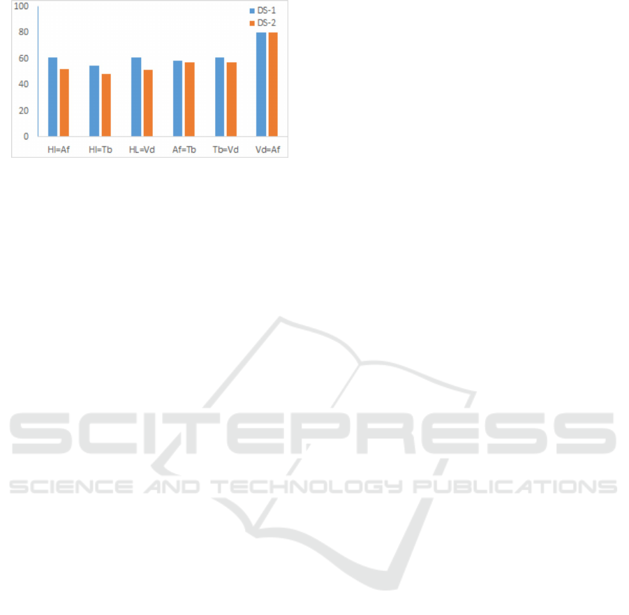
Figure 3: Percentages of tweets that are labelled with the

same sentiment label by the human labellers and the auto-

matic techniques: Aﬁnn, TextBlob and Vader.

‘HL=Tb’ and’ ‘HL=Vd’ represent the percentage of

labels that are the same across the human labelling

approach and the TextBlob labelling and Vader la-

belling respectively. The three automatic labelling

approaches: Aﬁnn, TextBlob and Vader obtain an av-

erage of 59% and 50.55% of equal sentiment labels

with the human labelling for DS-1 and DS-2 respec-

tively. On the other hand, there is a much higher

overlap of equal sentiment labels between Vader and

Aﬁnn (80%). We can also see in Figure 3 across the

different analyses and experiments that there is in-

consistency with the labels given by human labellers

and by the automatic labelling techniques with the

most agreement existing between Vader and Aﬁnn

labelling techniques. In Figure 3, there is, at best,

a difference of 41% (and sometimes more) between

the human labels and automatic labels. This explains

why the performance results in Experiment 3 are of-

ten poorer than those reported in Experiment 1 and 2.

The learning task is much more difﬁcult given that the

labels for the training data and the labels for the test

data are generated in different ways.

The best results are shown in Experiment 2 with

the automatic labelling approaches being used for

both the training and test sets. We argue that because

the same lexicon and rules have been used to label

both the training and test set it is easier for a ma-

chine learning approach to learn these rules and make

more accurate predictions. We suggest that this is not

the case with human labelling and hence the machine

learning models ﬁnd it more difﬁcult to do as well in

Experiment 1.

5 CONCLUSION

These experiments highlight the care that should be

taken in the use of both automatic and human la-

belling approaches. After evaluating both approaches,

we compared the performance of the three leading

automatic ternary labelling strategies to establish au-

tomatic labelling as a feasible alternative to human

labelling. This automated approach to sentiment la-

belling would yield extensive beneﬁts by eliminat-

ing the effort and cost of human labelling. Our re-

sults have identiﬁed the Aﬁnn approach as having the

highest level of labelling accuracy with both datasets.

We suggest that because both the training and test

sets were labelled with the same lexicon and rules,

a machine learning technique would ﬁnd it easier to

learn these rules and produce more accurate predic-

tions. These experiments motivate the need for fur-

ther investigations into the differences between the

different automatic approaches as well as the differ-

ences between human labelling and the automatic la-

belling approaches. However, the limitations of this

study include the potential mislabelling of data using

automated approaches. We have evaluated the exper-

iments on a relatively small size of the dataset with

only three labelling approaches, and this proposed

methodology might not be suitable where the train-

ing dataset is smaller than the testing dataset. In the

future, we want to continue this experiment for other

large text-classiﬁcation Twitter datasets, for example,

Covid19 or Covid-Vaccine related datasets. We will

also explore and extend this study to analyse the senti-

ment using other deep learning models with different

embedding methods, for example, BERT model with

word2vec and fast-text in the future. We hope these

studies would be helpful to analyse sentiment using

automatic labelling on large datasets when we want

to save time and cost for generating ground truth by

humans.

ACKNOWLEDGEMENTS

This work was supported by the College of Engineer-

ing, National University of Ireland, Galway.

REFERENCES

Camg

ozl

u, Y. and Kutlu, Y. (2020). Analysis of ﬁl-

ter size effect in deep learning. arXiv preprint

arXiv:2101.01115.

Chakraborty, K., Bhatia, S., Bhattacharyya, S., Platos, J.,

Bag, R., and Hassanien, A. E. (2020). Sentiment anal-

ysis of covid-19 tweets by deep learning classiﬁers—a

study to show how popularity is affecting accuracy in

social media. Applied Soft Computing, 97:106754.

Chaturvedi, I., Cambria, E., Welsch, R. E., and Herrera, F.

(2018). Distinguishing between facts and opinions for

sentiment analysis: Survey and challenges. Informa-

tion Fusion, 44:65–77.

DATA 2022 - 11th International Conference on Data Science, Technology and Applications

318

CrowdFlower (2016). https://www.ﬁgure-

eight.com/data/sentiment-analysis-emotion-text/.

Daniel, M., Neves, R. F., and Horta, N. (2017). Company

event popularity for ﬁnancial markets using twitter

and sentiment analysis. Expert Systems with Appli-

cations, 71:111–124.

Deepa, D., Tamilarasi, A., et al. (2019). Sentiment anal-

ysis using feature extraction and dictionary-based ap-

proaches. In 2019 Third International conference on I-

SMAC (IoT in Social, Mobile, Analytics and Cloud)(I-

SMAC), pages 786–790. IEEE.

Deriu, J. M., Gonzenbach, M., Uzdilli, F., Lucchi, A.,

De Luca, V., and Jaggi, M. (2016). Swisscheese at

semeval-2016 task 4: Sentiment classiﬁcation using

an ensemble of convolutional neural networks with

distant supervision. In Proceedings of the 10th inter-

national workshop on semantic evaluation (SemEval-

2016), pages 1124–1128.

Dimitrakakis, C. and Savu-Krohn, C. (2008). Cost-

minimising strategies for data labelling: optimal stop-

ping and active learning. In International Symposium

on Foundations of Information and Knowledge Sys-

tems, pages 96–111. Springer.

Hasan, A., Moin, S., Karim, A., and Shamshirband, S.

(2018). Machine learning-based sentiment analysis

for twitter accounts. Mathematical and Computa-

tional Applications, 23(1):11.

Hutto, C. and Gilbert, E. (2014). Vader: A parsimonious

rule-based model for sentiment analysis of social me-

dia text. In Proceedings of the international AAAI

conference on web and social media, volume 8, pages

216–225.

Lei, X., Qian, X., and Zhao, G. (2016). Rating prediction

based on social sentiment from textual reviews. IEEE

transactions on multimedia, 18(9):1910–1921.

Liao, S., Wang, J., Yu, R., Sato, K., and Cheng, Z. (2017).

Cnn for situations understanding based on sentiment

analysis of twitter data. Procedia computer science,

111:376–381.

Lindstrom, P., Delany, S. J., and Mac Namee, B. (2010).

Handling concept drift in a text data stream con-

strained by high labelling cost. In Twenty-Third In-

ternational FLAIRS Conference.

Mohammad, S., Kiritchenko, S., Sobhani, P., Zhu, X., and

Cherry, C. (2016). Semeval-2016 task 6: Detecting

stance in tweets. In Proceedings of the 10th inter-

national workshop on semantic evaluation (SemEval-

2016), pages 31–41.

Mohammad, S. M., Sobhani, P., and Kiritchenko, S. (2017).

Stance and sentiment in tweets. ACM Transactions on

Internet Technology (TOIT), 17(3):1–23.

Nielsen, F.

A. (2011). A new anew: Evaluation of a

word list for sentiment analysis in microblogs. arXiv

preprint arXiv:1103.2903.

Pennington, J., Socher, R., and Manning, C. D. (2014).

Glove: Global vectors for word representation. In

Proceedings of the 2014 conference on empirical

methods in natural language processing (EMNLP),

pages 1532–1543.

Poria, S., Cambria, E., and Gelbukh, A. (2015). Deep con-

volutional neural network textual features and multi-

ple kernel learning for utterance-level multimodal sen-

timent analysis. In Proceedings of the 2015 confer-

ence on empirical methods in natural language pro-

cessing, pages 2539–2544.

Saad, E., Din, S., Jamil, R., Rustam, F., Mehmood, A.,

Ashraf, I., and Choi, G. S. (2021). Determining the ef-

ﬁciency of drugs under special conditions from users’

reviews on healthcare web forums. IEEE Access,

9:85721–85737.

Sheng, V. S., Provost, F., and Ipeirotis, P. G. (2008). Get

another label? improving data quality and data min-

ing using multiple, noisy labelers. In Proceedings of

the 14th ACM SIGKDD international conference on

Knowledge discovery and data mining, pages 614–

622.

Snow, R., O’Connor, B., Jurafsky, D., and Ng, A. Y. (2008).

Cheap and fast–but is it good? evaluating non-expert

annotations for natural language tasks. In Proceed-

ings of the 2008 conference on empirical methods in

natural language processing, pages 254–263.

Turney, P. D. (1994). Cost-sensitive classiﬁcation: Empiri-

cal evaluation of a hybrid genetic decision tree induc-

tion algorithm. Journal of artiﬁcial intelligence re-

search, 2:369–409.

Wadera, M., Mathur, M., and Vishwakarma, D. K. (2020).

Sentiment analysis of tweets-a comparison of classi-

ﬁers on live stream of twitter. In 2020 4th Interna-

tional Conference on Intelligent Computing and Con-

trol Systems (ICICCS), pages 968–972. IEEE.

Whitehill, J., Wu, T.-f., Bergsma, J., Movellan, J., and Ru-

volo, P. (2009). Whose vote should count more: Op-

timal integration of labels from labelers of unknown

expertise. Advances in neural information processing

systems, 22.

Xu, G., Meng, Y., Qiu, X., Yu, Z., and Wu, X. (2019). Senti-

ment analysis of comment texts based on bilstm. IEEE

Access, 7:51522–51532.

Yoon, J. and Kim, H. (2017). Multi-channel lexicon inte-

grated cnn-bilstm models for sentiment analysis. In

Proceedings of the 29th conference on computational

linguistics and speech processing (ROCLING 2017),

pages 244–253.

A Comparison of Automatic Labelling Approaches for Sentiment Analysis

319