Using Video Motion Vectors for Structure from Motion 3D

Reconstruction

Richard N. C. Turner, Natasha Kholgade Banerjee and Sean Banerjee

Clarkson University, Potsdam, NY 13699, U.S.A.

Keywords:

H264, Structure from Motion, Motion Vectors, 3D Reconstruction.

Abstract:

H.264 video compression has become the prevalent choice for devices which require live video streaming and

include mobile phones, laptops and Micro Aerial Vehicles (MAV). H.264 utilizes motion estimation to predict

the distance of pixels, grouped together as macroblocks, between two or more video frames. Live video com-

pression using H.264 is ideal as each frame contains much of the information found in previous and future

frames. By estimating the motion vector of each macroblock for every frame, signiﬁcant compression can be

obtained. Combined with Socket on Chip (SoC) encoders, high quality video with low power and bandwidth

is now achievable. 3D scene reconstruction utilizing structure from motion (SfM) is a highly computational

intensive process, typically performed ofﬂine with high computing devices. A signiﬁcant portion of the com-

putation required for SfM is in the feature detection, matching and correspondence tracking necessary for the

3D scene reconstruction. We present a SfM pipeline which uses H.264 motion vectors to replace much of the

processing required to detect, match and track correspondences across video frames. Our pipeline results have

shown a signiﬁcant decrease in computation, while accurately reconstructing a 3D scene.

1 INTRODUCTION

3D reconstruction of a video scene using structure

from motion (SfM) is a highly challenging problem

when using existing techniques (Resch et al., 2015).

Full motion video can produce thousands of overlap-

ping images in just a few seconds of video. Fur-

thermore, high resolution images numbering in the

thousands further challenge the efﬁciency of feature

detection and matching algorithms needed for corre-

spondence searching. Combined, the difﬁculties with

processing a single video can become insurmount-

able without a means to ﬁlter the overlapping scenes.

A common technique for frame ﬁltering is to select

keyframes found in the video sequence (Hwang et al.,

2008; Whitehead and Roth, 2001). However, selec-

tion of keyframes which would generate an accurate

3D scene reconstruction is difﬁcult as information be-

tween keyframes is lost. Subsequently, increasing en-

coded keyframes to account for the loss of informa-

tion will signiﬁcantly impact video streaming band-

width and compression, making this technique for

SfM undesirable in full motion video streaming (Ed-

palm et al., 2018).

Our approach leverages the inherit video compres-

sion of H.264 and its encoded Motion Vector Distance

(MVD) to process the information which would oth-

erwise be lost between keyframes. Starting with fea-

ture detection of the keyframe, we suggest the mo-

tion vectors between subsequent inter frames can be

used to accurately predict the matching of said fea-

tures over time. Furthermore, correspondence match-

ing and tracking between inter and keyframes can be

accomplished with a unique feature map. A predeter-

mined frame interval is used to narrow the ﬁnal views

for incremental reconstruction. Our approach does

not require the sub-sampling of video for frame ﬁlter-

ing or image resolution. Instead, we leverage the in-

herit video compression algorithms already in use for

live video streaming to perform the majority of corre-

spondence searching and tracking. We validated our

pipeline with video taken from a MAV ﬂying within

an urban environment (Majdik et al., 2017).

2 RELATED WORK

H.264 is a hybrid block encoder which relies on the

prediction of macroblocks between frames to provide

much of its compression (Richardson, 2010). Mo-

tion estimation techniques are integral to the perfor-

mance of H.264 video compression prediction (Man-

Turner, R., Banerjee, N. and Banerjee, S.

Using Video Motion Vectors for Structure from Motion 3D Reconstruction.

DOI: 10.5220/0011263600003289

In Proceedings of the 19th International Conference on Signal Processing and Multimedia Applications (SIGMAP 2022), pages 13-22

ISBN: 978-989-758-591-3; ISSN: 2184-9471

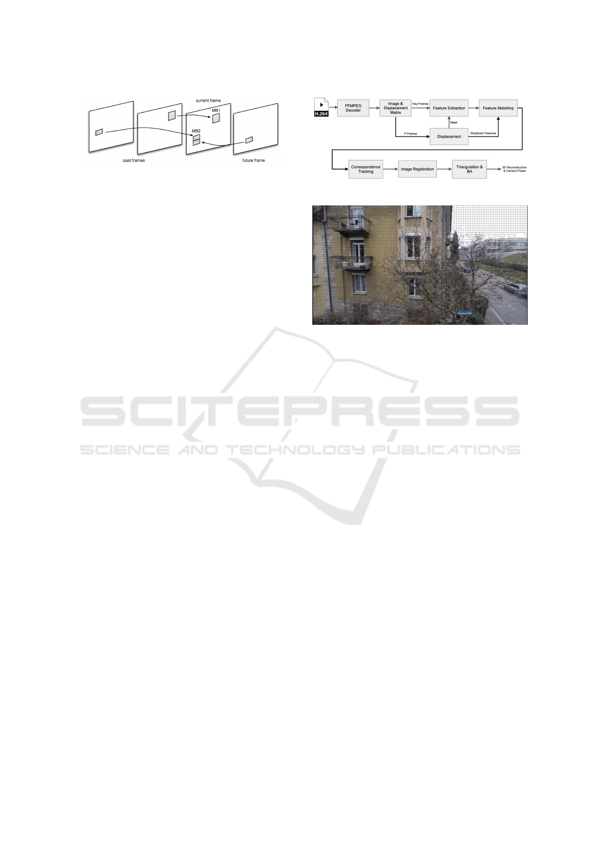
Figure 1: Inter-frame prediction of H.264 video compres-

sion.

cas et al., 2012), as they allow for the encoding of

motion between frames, called motion vectors, with-

out having to fully encode every frame. Each frame

is broken down into one of three types—P-frames,

B-frames and keyframes, also known as reference

frames or Intra-frames. P-frames and B-frames are

predicted inter-frames from another frame, as shown

by the ﬂowchart in Figure 1. Keyframes are full

frames that do not rely on inter-frame motion esti-

mation for decoding. The collection of frames to-

gether form a Group of Pictures (GOP). The length

of each GOP is dependent on many factors includ-

ing scene changes and error resiliency between pre-

dictions. Typically for live video, the increase in

keyframes will subsequently increase the video com-

pression size and bandwidth for transmission. Ideally,

you want to have a good balance of GOP size of the

video to maintain quality while also increasing com-

pression.

SfM is a pipeline which provides 3D reconstruc-

tion of a scene starting with a collection of images

(Bianco et al., 2018). The collection of steps for a

SfM pipeline typically involves feature detection, fea-

ture matching, correspondence tracking, image reg-

istration, triangulation, bundle adjustment, and point

cloud generation. Collectively each has their own

methods and algorithms which contribute to the ac-

curacy, efﬁciency and completeness of the ﬁnal 3D

reconstruction. While many SfM pipelines can han-

dle large collection of images, video provides a new

challenge for SfM reconstruction.

SfM reconstruction using video is a growing re-

search area, with varying degrees of success and

methods when applied to unstructured scenes. Bros-

tow et al. (2008) derived 3D point clouds using

ego-motion, although the processing is done ofﬂine.

Scene detection using H.264 motion estimation has

been used for foreground and background detection.

Laumer et al. (2016) used the macroblocks between

frames as masks to determine depth of the frame,

and Vacavant et al. (2011) used the size of the mac-

roblock to create background models of the scene.

Yoon and Kim (2015) proposed a prediction struc-

tures of a scene using a hierarchical search strategy

derived from video compression motion vectors. Fur-

thermore, Shum et al. (1999) used virtual keyframes

Figure 2: Motion vector pipeline for SfM reconstruction.

Figure 3: Visual motion vectors over one scene in the ex-

perimental data set.

for multi-frame SfM reconstruction. Our method fo-

cuses on the use of live video streams with their mo-

tion vector distances providing forward predicted fea-

tures across a given scene. Our experimental results

show a SfM reconstruction that is accurate, robust and

highly efﬁcient across varying environments.

3 MOTION VECTOR PIPELINE

Our approach for 3D reconstruction of a video scene

was to build a highly capable pipeline within the

OpenMVG framework, as shown by the ﬂowchart in

Figure 2. OpenMVG is the ideal library for this ef-

fort as it makes available a number of easy to use

SfM tools and pipelines with an active community

base (Moulon et al., 2016). We modiﬁed the exist-

ing incremental pipeline within OpenMVG to pro-

vide video decoding using the FFMPEG application,

robust feature extraction and motion vector distance

algorithm for two types of video frames—keyframes

and P-frames, feature matching across keyframes and

P-frames, and a dynamic correspondence tracker.

3.1 Motion Vector Encoding

Motion vectors are used to represent the macroblocks

in a video frame and are computed based on the posi-

tion of a macroblock in the current frame, sometimes

called the target frame, to its reference frame (Bakas

et al., 2021). Motion vectors can be visually repre-

sented, where the length and direction of the vector

SIGMAP 2022 - 19th International Conference on Signal Processing and Multimedia Applications

Figure 4: MVD matrix used for forward motion prediction

of detected features.

drawn is determined by the MVD from the reference

to target frame, as shown by the image in Figure 3.

For each inter-frame, a collection of motion vectors

are computed using a motion prediction algorithm

within the video encoder. For our research we in-

vestigated a number of motion prediction algorithms

available for H.264 including brute force, bounding

box, and hex searching. The search radius is con-

ﬁgured by a pixel boundary, where the center of the

reference macroblock is the start and the range of the

motion estimation matching is clamped to a speciﬁc

limit within the target frame. We have found using a

complex multi-hexagon search pattern with a search

radius of 32 pixels to be optimal for our purposes.

B-frames, or bi-directional inter-frames, are not sup-

ported within the motion vector pipeline, therefore B-

frames were not included in the transcoding of images

from the video data set.

3.2 Motion Vector Difference (MVD)

Matrix

To ﬁnd the MVD between the reference frame and the

target frame we extract the motion vector side data

during frame decoding. Decoded motion vector side

data is an array structure containing the difference for

each macroblock for a given video frame. Given the

motion vector target (MV

)) and reference (MV

)) x

and y values, the corresponding difference is deﬁned

= MV

x − MV

x, and (1)

= MV

y − MV

y. (2)

The difference (D

, D

) is calculated as the centroid

of the macroblock. For every frame a MVD matrix

is created, with equal width and height as the frame.

The calculated difference value is stored in the MVD

matrix with a given area equal to the macroblock size,

as shown by the MVD matrix in Figure 4. The mac-

roblock highlighted is a 4×4 block size with a pre-

vious frame pixel difference of 2.0 pixels along the x

axis and -3.2 pixels along the y axis.

In addition to the MVD matrix, every frame has

a calculated macroblock coverage area. Given the

width w

and height h

for each macroblock, the cal-

culated coverage area (C) for any frame is deﬁned as

C =

k−1

∑

i=0

(3)

where k is the current macroblock for a given frame,

F is the frame. The equation deﬁnes the coverage

area C as the ratio of the total coverage area to the

total frame area. Coverage area is used during fea-

ture detection to determine if the macroblocks for a

given frame is below a certain deﬁned threshold and

therefore should have their features detected using a

macroblock binary mask.

3.3 Feature Detection

For every keyframe, a feature detection algorithm is

used to identity as many potential correspondences

for further matching. Although the pipeline can be ran

with different feature detection algorithms, we have

found the best possible results using the Accelerated-

KAZE algorithm (Alcantarilla et al., 2013) at the

highest describe preset. For every feature detected, a

unique feature identiﬁer is created and stored within a

feature mapping, where the map identiﬁer is a unique

feature id and the value is a list of matching views. A

view consists of a unique identiﬁer, image frame, fea-

tures and descriptors, MVD matrix, macroblocks, and

the macroblock total coverage area. The feature map

is used to determine correspondence tracking across

views.

For P-frames, the previous view feature locations

are updated using the current view MVD matrix. Pre-

vious views can be either keyframes or P-frames. Any

features displaced out of the view area are removed

from the current view list of features. We are able to

achieve feature tracking across the views by adjust-

ing the previous view features with the current view

MVD matrix, as shown by the two images in Figure 5.

Frame 1 has detected the pole connector to the build-

ing. After 250 frames and an x axis distance of over

350 pixels, the feature was tracked accurately. Fea-

ture map entries for all features of the current view

are updated with the current view identiﬁer, thereby

matching previous view features to current view fea-

tures.

The ability to apply feature motion vectors be-

tween views is dependent on the H.264 encoding al-

gorithms ability to determine the matching of mac-

roblocks between frames. When encoding H.264 with

non-deterministic GOP length, the expectation of a

keyframe cannot be predicted. In our experimental

data set at 30 frames per second (FPS), we ﬁnd GOP

Using Video Motion Vectors for Structure from Motion 3D Reconstruction

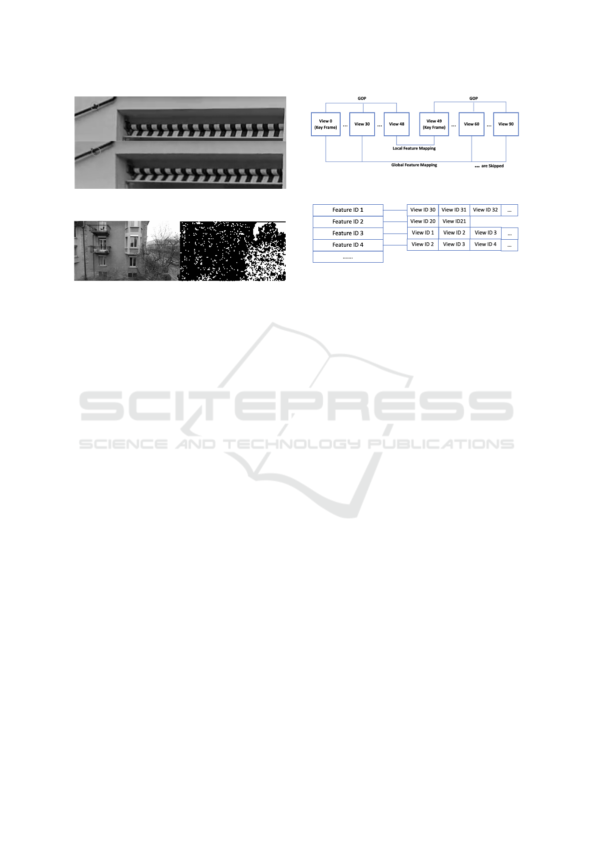
Figure 5: Feature detection and correspondence between

250 frames.

Figure 6: Frame and macroblock coverage area of a frame

with less than 70% coverage for their macroblocks.

lengths averaging 240 frames between keyframes.

Hence, we need to account for any reduction in mac-

roblock coverage when a keyframe is not available.

The ability of the encoding algorithm to determine

previous macroblocks for a P-frame is impacted by

many factors such as changes in the camera pose, oc-

clusion from a new object within the scene, and lu-

minance changes to name a few. For these reasons,

we use the total coverage area of the view to deter-

mine if a predetermined coverage threshold has been

met. We have found a threshold of 70% coverage to

be optimal for the experimental data set. A low cov-

erage area will eventually result in further ﬁltering of

subsequent features until a new keyframe is received.

To account for this reduction, any P-frame below the

threshold will have feature detection performed with

a calculated mask. The mask is a binary image of

the null space which shouldn’t be used for feature de-

tection, thereby reducing signiﬁcantly the processing

time required. The mask is calculated from the cur-

rent view macroblock areas, as shown by the image

and binary mask in Figure 6. The frame on the left

introduced a new occluding object, the tree located

at the bottom right of the frame, whereas the frame

on the right shows the macroblock coverage in black.

The resulting total macroblock coverage area is be-

low the threshold, thereby requiring feature detection

on the new occluding object.

3.4 Feature Matching

Feature matching is performed in two stages, global

and local, as shown by ﬂowchart in Figure 7. Global

feature matching is predominately performed with the

use of the feature map in feature detection. At the

Figure 7: Local and global feature matching at 30 FPS for

3 Sec. video.

Figure 8: Feature map strcuture to track each view for a

given feature. Used during feature detection and matching.

conclusion of feature detection, association between

the views and the features is complete, as shown by

the feature mapping in Figure 8. With the possibili-

ties of thousands of views for further incremental pro-

cessing, a reduction of the views is needed. For this

we use the video FPS as the skip factor for the views.

At 30 FPS for a 60 second video, we ﬁlter 1800 views

down to a minimum of 60 views for incremental pro-

cessing. Localized feature matching will increase the

ﬁnal view count. Only the features matching between

the selected views will be carried forward as tracks.

Thus, the features which have short lifespans will be

eliminated. A higher FPS will result in a higher conﬁ-

dence level for the selection of tracks found between

the selected views, thereby stabilizing the ﬁnal 3D re-

construction.

Inherently there is a feature matching gap be-

tween the last P-frame of a GOP and the following

keyframe. Global feature matching will only build

the tracks within each GOP, as the process of fea-

ture detection and matching is restarted after every

keyframe. For this reason we perform a local one-

to-one feature match between the last P-frame of the

GOP and the following keyframe. Localized fea-

ture matching between the two views is done using

a cascade hashing matching algorithm (Cheng et al.,

2014). The P-frame and keyframe with their matched

features are added to the ﬁnal views and tracks for

incremental processing. Lastly, a geometric feature

ﬁltering using direct linear transform (DLT) is per-

formed on all selected views and their matched fea-

tures (Hartley and Zisserman, 2004). This last step

will remove any remaining outliers outside of the ro-

bust model estimate.

The use of multi-threading libraries such as

OpenMP (Dagum and Menon, 1998) for feature

matching results in signiﬁcant performance increases

SIGMAP 2022 - 19th International Conference on Signal Processing and Multimedia Applications

Figure 9: Example frame subset 36:00 to 36:30 from the

experimental data set.

(Pang et al., 2020). For our feature matching, the fea-

ture map data is reﬁned to a set of correspondences for

each view, whereby the correspondences are paired

with matching views to form tracks. The process of

generating the pairing is performed using OpenMP,

thereby signiﬁcantly decreasing the feature matching

execution time. The resulting tracks is sent to the in-

cremental pipeline for further SfM reconstruction.

4 EXPERIMENTAL EVALUATION

We compare the execution time and accuracy of fea-

ture detection and matching using our approach and

two methods using only keyframes—deterministic

GOP with one keyframe per second and non-

deterministic GOP where the keyframe is determined

by the compression algorithm. We have identi-

ﬁed these three methods as Motion Vector Track-

ing (MVT), Deterministic GOP (DGOP), and Non-

Deterministic GOP (N-DGOP) respectively.

DGOP is the most common technique used today

in extracting frames for feature extraction (Nixon and

Aguado, 2012). Keyframe selection is determined by

either the length of the video as a keyframe selection

percentage selection or using the Frames Per Second

(FPS) as a deterministic selection. For example, an

FPS of 30 would determine the keyframe selection as

one frame every 30 frames, irregardless of scene con-

tent. N-GOP relies on the video coding compression

algorithm to determine the placement of keyframes.

Scenes with minimal movement results in a longer

GOP length, while a dynamic scene would result in

a shorter GOP length. N-DGOP is rarely used today

due to the irregular GOP length and the necessity to

capture scene changes that would otherwise not pro-

duce a keyframe.

Our method is the best of both DGOP and N-

DGOP. We take advantage of the video encoding al-

gorithms ability to adjust GOP length dependent on

scene changes as seen in N-GOP. The downsides of

N-DGOP such as of longer GOP lengths is signiﬁ-

cantly reduced in our algorithm by using MVD for

feature matching and tracking along with the mac-

roblock coverage area calculations to detect smaller

scene changes. The ﬁnal selection of tracks in our

algorithm takes advantage of the DGOP method, by

ﬁltering the tracking window to a ﬁxed FPS.

The experimental data was taken from (Majdik

et al., 2017), where the 81,000 images at a resolu-

tion of 1920×1080, were pre-processed using FFM-

PEG into 30 second subsets. Prior to pre-processing,

the intrinsic parameters were calculated using the ref-

erence calibration images found in the experimental

data. Furthermore, any image distortions were re-

moved using Matlab.

For the MVT dataset, the framerate is set at 30

FPS with only keyframes and P-frames, generating

on average 900 frames per subset. For the N-DGOP

dataset, the frame rate is set at 30 FPS with keyframes,

P-frames and B-frames, generating on average 900

frames per subset. Lastly, the frame rate of DGOP

dataset is set at 1 FPS with only keyframes, generating

30 frames per subset. All experiments are performed

on a Dell Precision 7550 Laptop running Ubuntu

20.04 with 32GB of main memory, 1TB NVMe drive

and an i7-1087 processor.

4.1 Feature Detection and Matching

We compare the execution time for feature detection

and matching using MVT, DGOP and N-DGOP. All

experiments utilize the A-KAZE feature extractor al-

gorithm with the highest describer preset available

in OpenMVG. Feature detection is a major operation

within any SfM pipeline, resulting in signiﬁcant ex-

ecution penalties for each image processed (Kalms

et al., 2017). MVT and N-DGOP perform feature

detection on each keyframe, typically 3-4 frames for

each 30 second subset. NGOP incurs the highest

penalty in execution time as the number of keyframes

are ﬁxed at 1 frame per second, or 30 frame for each

30 second subset. On average our approach of MVT

is 2.8 times faster than DGOP and slightly slower

than N-DGOP when performing feature detection, as

shown by the graph in Figure 10. Whereas N-DGOP

only performs feature detection on each keyframe

without inter-frame detection, MVT performs addi-

tional calculations on each P-frame to displace the

features across frames, thereby providing a robust fea-

ture matching for every frame with limited execution

penalty.

The signiﬁcant differences in execution time be-

tween MVT and DGOP become evident during fea-

ture matching. Whereas our approach inherently per-

Using Video Motion Vectors for Structure from Motion 3D Reconstruction

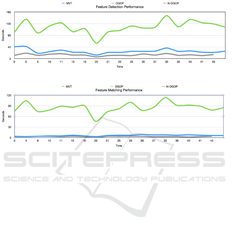
Figure 10: Feature detection execution time for each minute where all three methods are captured over the entire 45 minute

data set.

Figure 11: Feature matching execution time for each minute where all three methods are captured over the entire 45 minute

data set. MVT outperforms DGOP by a signiﬁcant factor.

forms the majority of feature matching during fea-

ture detection when creating the feature map, DGOP

needs to execute feature matching on an exhaustive

list of feature pairs, utilizing both putative and geo-

metric ﬁltering. Our approach only needs to perform

feature matching with localized keyframes, inter-

frame matching is done through global feature map-

ping with the use of the feature map. Our approach

is on average 9.2 times faster in execution time than

DGOP, as shown by the graph in Figure 11. In to-

tal, the execution time of MVT is close to the FPS

execution time, thereby providing a near real-time ex-

ecution of feature detection and matching when pro-

cessing video.

4.2 SfM Reconstruction

As shown by the image in Figure 9, the landmarks

are predominately buildings and streets with an ex-

ceedingly high number of features within each scene.

It is obvious for the scene to accurately generate a

sparse point cloud, the pipeline will need a high num-

ber of tracks to account for the high number of fea-

tures across each subset.

In order to demonstrate the SfM reconstruc-

tion, all subsets are processed using an incremen-

tal pipeline at the conclusion of feature matching

and tracking. Identical threshold parameters for the

pipeline are used for MVT, DGOP anxd N-DGOP.

The subset SfM reconstruction results, which are pro-

cessed in 30 second increments, are collected and av-

eraged across 2.5 minute slices as seen in Table 1 and

Table 2. Table 1 shows the median, maximum and

mean error residual during non-linear bundle adjust-

ment for MVT, DGOP and N-DGOP. The lower the

error residual, the lower the reprojection difference

during image registration. Table 2 shows the regis-

tered poses, tracks and SfM points averaged across

each 2.5 minute slice.

During SfM triangulation and BA, scenes and

tracks are reﬁned in order to minimize the residual

reprojection cost. BA reﬁnes the 3D reconstruction

to produce an optimal structure and pose estimate

(Triggs et al., 1999). By default, OpenMVG will

constrain the maximum pixel reprojection error to a

residual threshold, defaulting to 4.0 pixels as shown

in Table 1. On average, the residual mean for MVT

is twice as high to the residual mean for DGOP and

N-DGOP, as shown by the graph in Figure 13. This

is most likely a result of drift, resulting from mo-

tion vector distance accuracy of the features across

the frames. Reducing the search radius boundary of

SIGMAP 2022 - 19th International Conference on Signal Processing and Multimedia Applications

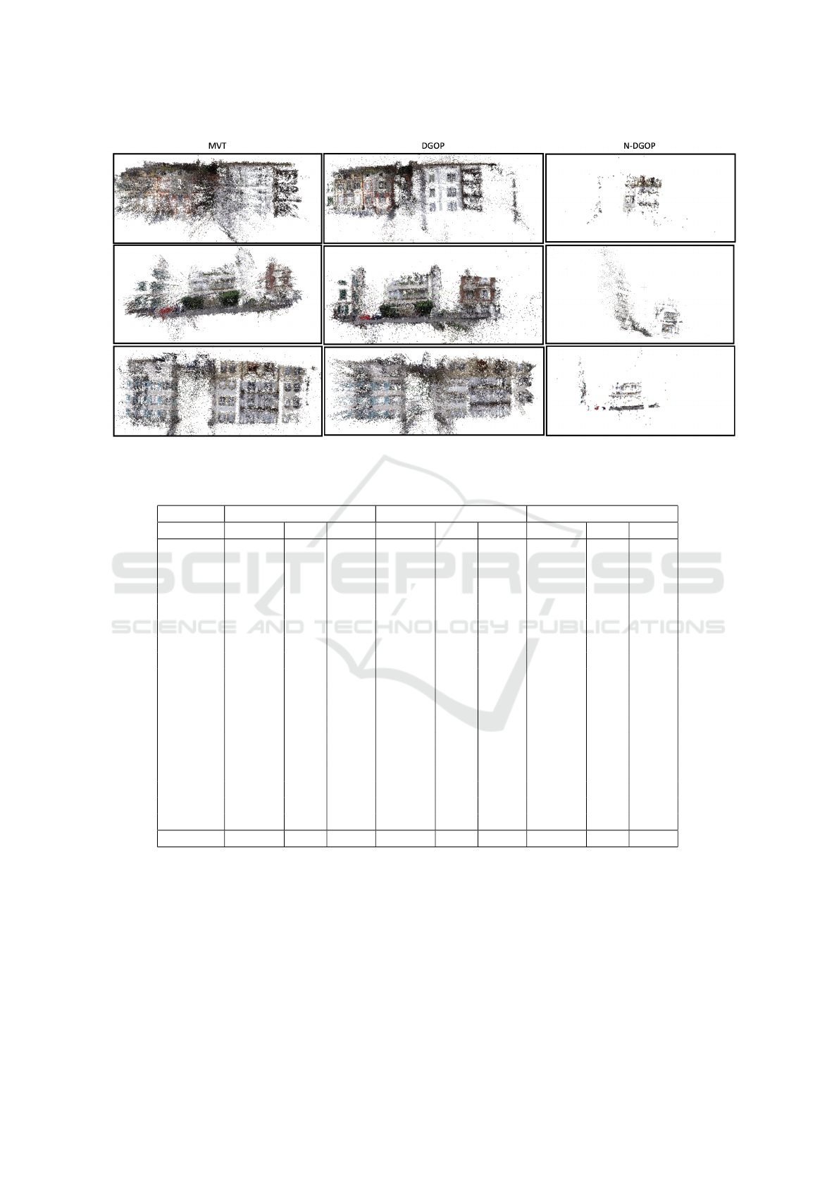
Figure 12: Sparse SfM reconstruction subsets for MVT, DGOP and N-DGOP.

Table 1: Summary of SfM residual results across all subsets. Average taken every 2.5 minutes.

Subsets MVT Residuals DGOP Residuals N-DGOP Residuals

Median Max Mean Median Max Mean Median Max Mean

0 - 2.5 0.87 3.99 1.05 0.30 3.98 0.54 0.32 3.87 0.49

2.5 - 5 0.75 3.98 0.95 0.33 3.99 0.51 0.08 3.73 0.22

5 - 7.5 0.74 3.98 0.96 0.31 3.99 0.52 0.10 3.96 0.40

7.5 - 10 0.84 3.99 1.02 0.34 3.98 0.55 0.18 3.93 0.42

10 - 12.5 0.85 3.99 0.97 0.31 3.98 0.52 0.23 3.99 0.42

12.5 - 15 0.86 3.99 1.04 0.32 3.99 0.52 0.17 3.97 0.42

15 - 17.5 0.82 3.99 1.01 0.26 3.99 0.45 0.19 3.99 0.41

17.5 - 20 0.87 3.99 0.98 0.34 3.99 0.56 0.19 3.99 0.42

20 - 22.5 0.95 3.99 1.10 0.41 3.99 0.68 0.28 3.87 0.41

22.5 - 25 0.90 3.99 1.09 0.29 3.98 0.49 0.18 3.83 0.44

25 - 27.5 0.93 3.99 1.11 0.33 3.98 0.54 0.20 3.98 0.45

27.5 - 30 0.86 3.99 1.04 0.26 3.99 0.42 0.19 3.99 0.41

30 - 32.5 0.89 3.99 1.07 0.26 3.99 0.46 0.28 3.99 0.40

32.5 - 35 0.83 3.98 1.02 0.28 3.98 0.46 0.21 3.99 0.43

35 - 37.5 0.86 3.99 1.05 0.32 3.98 0.50 0.30 3.97 0.45

37.5 - 40 0.80 3.99 1.00 0.40 3.98 0.55 0.29 3.99 0.44

40 - 42.5 0.87 3.99 0.98 0.42 3.99 0.56 0.21 3.99 0.40

42.5 - 45 0.78 3.99 0.97 0.39 3.99 0.50 0.21 3.99 0.40

Avg 0.85 3.99 1.02 0.33 3.99 0.52 0.21 3.95 0.41

the motion prediction may result in a lower residual

threshold. From manual observation of the generated

sparse point cloud, we have found the resulting re-

construction for MVT to be within an acceptable ac-

curacy.

The 3D reconstructed sparse point cloud is con-

structed from the poses of each view along with the

3D tracks across the scene. MVT reconstruction of

the sparse point cloud follows the same pattern of re-

constructed points as DGOP, generating comparable

and sometimes exceeding the reconstructed points,

as shown by the graph in Figure 14. On average,

36 poses are used for MVT reconstruction while 30

poses are used for DGOP, as seen in Table 2. The rea-

son for the increase in poses for MVT is due to the

local feature matching of the last GOP frame to the

subsequent keyframe.

An example SfM reconstruction of a sparse point

Using Video Motion Vectors for Structure from Motion 3D Reconstruction

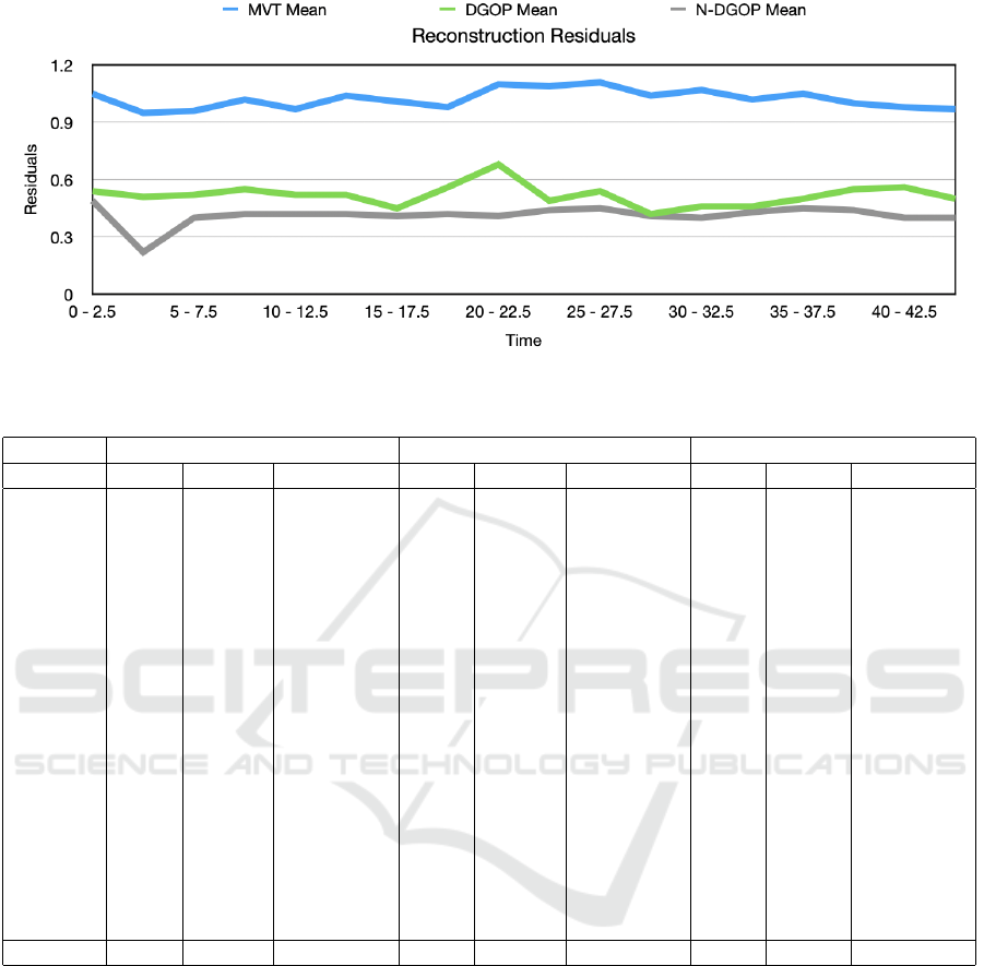
Figure 13: Reconstructed residuals across all subsets. Average taken every 2.5 minutes.

Table 2: Summary of SfM sparse point cloud results across all subsets. Average taken every 2.5 minutes.

Subsets MVT DGOP N-DGOP

Poses Tracks SfM Points Poses Tracks SfM Points Poses Tracks SfM Points

0 to 2.5 36 172550 48970 30 79149 21009 4 9313 8296

2.5 - 5 35 173580 85902 30 105869 83099 3 8126 6452

5 - 7.5 35 160546 73189 30 123035 87439 4 5172 4951

7.5 - 10 35 176733 68361 30 90142 61874 4 3961 3391

10 - 12.5 36 186946 102120 30 92946 60010 4 3920 3644

12.5 - 15 36 176655 130502 30 122431 113731 4 6659 6404

15 - 17.5 36 164114 81464 30 126910 117156 3 2538 2202

17.5 - 20 36 110933 74948 30 76241 67235 4 4388 4148

20 - 22.5 36 168764 96690 30 74033 53990 4 4062 3119

22.5 - 25 36 170314 125541 30 135818 121075 4 2625 2539

25 - 27.5 36 182639 131164 30 133942 109486 4 3988 3420

27.5 - 30 36 193579 150827 30 152141 136585 4 4993 4489

30 - 32.5 36 192626 152862 30 134933 122653 4 3791 3562

32.5 - 35 35 186762 88008 30 98458 80316 4 2988 2691

35 - 37.5 36 180705 138438 30 115189 98574 4 4165 3998

37.5 - 40 36 163298 73395 30 86668 70094 4 2779 2109

40 - 42.5 36 187044 129193 30 104809 84331 4 3099 2691

42.5 - 45 36 179906 105934 30 95614 74091 4 2971 2509

Avg 36 173761 103195 30 108240 86819 4 4419 3923

cloud for all three methods can be found in Figure

12. As shown, the generated sparse point cloud for N-

DGOP is unrecognizable, which is evident with their

low average number of SfM points at 3,923. Even

though N-DGOP has a low execution time, the inabil-

ity to generate an accurate sparse point cloud removes

this method as a viable candidate. Using visual anal-

ysis, both MVT and DGOP are able to generate a rep-

resentation of the video scene. MVT generates on av-

erage 15% more SfM points than DGOP, although the

residuals of DGOP are half that of MVT. Given low

execution time of MVT compared to DGOP, and abil-

ity to generate a stable sparse point cloud, MVT is

ideal for live video scene SfM reconstruction.

5 DISCUSSION

Our method relies on a ﬁxed skip factor using video

FPS for the matching of features across frames. Fea-

tures which exhibit strong correlation between frames

are lost if they don’t extend past the skip factor. As

future work it would be preferably to analyze the

strength of correlation between features as a means

for determining inclusion in the ﬁnal track set. In ad-

dition, keyframe selection on a sliding window for lo-

cal BA could be implemented (Strasdat et al., 2012).

Moreover, our algorithm is executed using CPU and

system memory. Improvements in execution time can

be made if implemented using a low-grade GPU.

SIGMAP 2022 - 19th International Conference on Signal Processing and Multimedia Applications

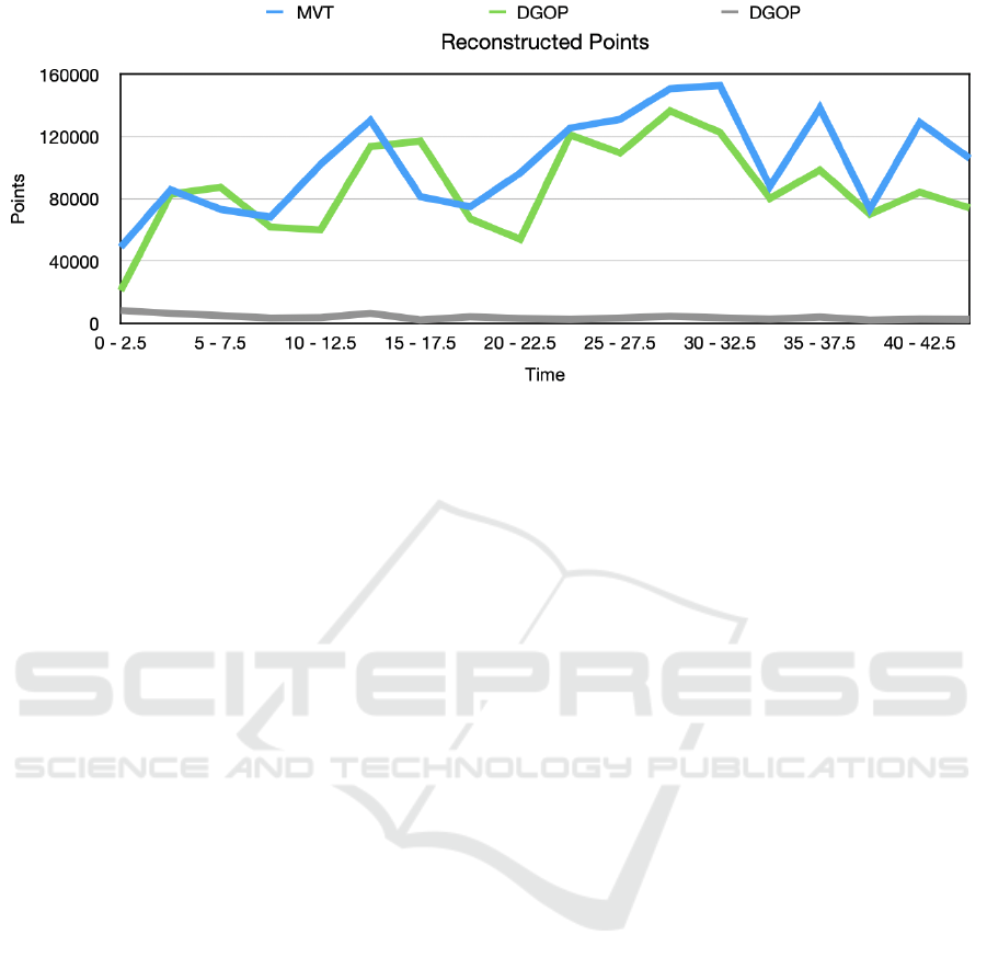
Figure 14: Reconstructed points across all subsets. Average taken every 2.5 minutes.

In future work, the inclusion of B-frames should

be implemented to further take advantage of video

compression motion estimation for feature detection

and matching. Moreover, further research of our ap-

proach with additional SfM pipelines should be pur-

sued to include simultaneous localization and map-

ping (SLAM) techniques.

6 CONCLUSION

This paper introduces a near real-time feature detec-

tion and matching algorithm for SfM reconstruction

using the properties of motion estimation found in

H.264 video compression encoders. Utilizing the mo-

tion vectors of the compressed video frames, we can

accurately predict the matching of features between

frames over time. The design has been evaluated

against multiple extraction techniques using an identi-

cal incremental pipeline to generate a 3D sparse point

cloud. In comparison, we have found our approach to

have very low execution time while also balancing the

accuracy of the generated sparse point cloud.

REFERENCES

Alcantarilla, P. F., Nuevo, J., and Bartoli, A. (2013). Fast

explicit diffusion for accelerated features in nonlin-

ear scale spaces. In British Machine Vision Conf.

(BMVC).

Bakas, J., Naskar, R., and Bakshi, S. (2021). Detection and

localization of inter-frame forgeries in videos based

on macroblock variation and motion vector analysis.

Computers and Electrical Engineering, 89:106929.

Bianco, S., Ciocca, G., and Marelli, D. (2018). Evaluating

the performance of structure from motion pipelines.

Journal of Imaging, 4:98.

Brostow, G. J., Shotton, J., Fauqueur, J., and Cipolla, R.

(2008). Segmentation and recognition using struc-

ture from motion point clouds. In Forsyth, D.,

Torr, P., and Zisserman, A., editors, Computer Vi-

sion – ECCV 2008, pages 44–57, Berlin, Heidelberg.

Springer Berlin Heidelberg.

Cheng, J., Leng, C., Wu, J., Cui, H., and Lu, H. (2014).

Fast and accurate image matching with cascade hash-

ing for 3d reconstruction. In Proceedings of the IEEE

conference on computer vision and pattern recogni-

tion, pages 1–8.

Dagum, L. and Menon, R. (1998). Openmp: an industry

standard api for shared-memory programming. IEEE

computational science and engineering, 5(1):46–55.

Edpalm, V., Martins, A., Maggio, M., and rzn, K.-E. (2018).

H.264 video frame size estimation. Technical report,

Department of Automatic Control, Lund Institute of

Technology, Lund University.

Hartley, R. and Zisserman, A. (2004). Multiple View Geom-

etry in Computer Vision. Cambridge University Press,

2 edition.

Hwang, Y., Seo, J.-K., and Hong, H.-K. (2008). Key-frame

selection and an lmeds-based approach to structure

and motion recovery. IEICE Transactions, 91-D:114–

123.

Kalms, L., Mohamed, K., and G

ohringer, D. (2017). Accel-

erated embedded akaze feature detection algorithm on

fpga. Proceedings of the 8th International Symposium

on Highly Efﬁcient Accelerators and Reconﬁgurable

Technologies.

Laumer, M., Amon, P., Hutter, A., and Kaup, A. (2016).

Moving object detection in the h.264/avc compressed

domain. APSIPA Transactions on Signal and Informa-

tion Processing, 5:e18.

Majdik, A., Till, C., and Scaramuzza, D. (2017). The zurich

urban micro aerial vehicle dataset. The International

Journal of Robotics Research, 36:027836491770223.

Mancas, M., Beul, D. D., Riche, N., and Siebert, X. (2012).

Human attention modelization and data reduction. In

Punchihewa, A., editor, Video Compression, chap-

ter 6. IntechOpen, Rijeka.

Using Video Motion Vectors for Structure from Motion 3D Reconstruction

Moulon, P., Monasse, P., Perrot, R., and Marlet, R. (2016).

OpenMVG: Open multiple view geometry. In Interna-

tional Workshop on Reproducible Research in Pattern

Recognition, pages 60–74. Springer.

Nixon, M. and Aguado, A. S. (2012). Feature Extraction &

Image Processing for Computer Vision, Third Edition.

Academic Press, Inc., USA, 3rd edition.

Pang, Q., Gui, J., Jing, L., and Deng, B. (2020). Fast 3d re-

construction based on uav image. Journal of Physics:

Conference Series, 1693:012172.

Resch, B., Lensch, H. P. A., Wang, O., Pollefeys, M., and

Sorkine-Hornung, A. (2015). Scalable structure from

motion for densely sampled videos. In 2015 IEEE

Conference on Computer Vision and Pattern Recog-

nition (CVPR), pages 3936–3944.

Richardson, I. E. (2010). The H.264 Advanced Video Com-

pression Standard. Wiley Publishing, 2nd edition.

Shum, H.-Y., Ke, Q., and Zhang, Z. (1999). Efﬁcient bundle

adjustment with virtual key frames: a hierarchical ap-

proach to multi-frame structure from motion. In Pro-

ceedings. 1999 IEEE Computer Society Conference

on Computer Vision and Pattern Recognition (Cat. No

PR00149), volume 2, pages 538–543 Vol. 2.

Strasdat, H. M., Montiel, J. M. M., and Davison, A. J.

(2012). Visual slam: Why ﬁlter? Image Vis. Com-

put., 30:65–77.

Triggs, B., McLauchlan, P. F., Hartley, R. I., and Fitzgibbon,

A. W. (1999). Bundle adjustment - a modern synthe-

sis. In Proceedings of the International Workshop on

Vision Algorithms: Theory and Practice, ICCV ’99,

page 298372, Berlin, Heidelberg. Springer-Verlag.

Vacavant, A., Robinault, L., Miguet, S., Poppe, C., and

Van de Walle, R. (2011). Adaptive background sub-

traction in h. 264/avc bitstreams based on macroblock

sizes. In VISAPP, pages 51–58.

Whitehead, A. and Roth, G. (2001). Frame extraction for

structure from motion. National Research Council of

Canada.

Yoon, H. and Kim, M. (2015). Temporal prediction struc-

ture and motion estimation method based on the char-

acteristic of the motion vectors. Journal of Korea Mul-

timedia Society, 18:1205–1215.

SIGMAP 2022 - 19th International Conference on Signal Processing and Multimedia Applications