Solving Stable Generalized Lyapunov Equations for Hankel Singular
Values Computation
Vasile Sima
a
Technical Sciences Academy of Romania, Bucharest, Romania
Keywords:
Balancing, Hankel Singular Values, Lyapunov Equation, Numerical Methods, Stability.
Abstract:
Generalized Lyapunov equations are often encountered in systems theory, analysis and design of control sys-
tems, and in many applications, including balanced realization algorithms, procedures for reduced order mod-
els, or Newton methods for generalized algebraic Riccati equations. An important application is the computa-
tion of the Hankel singular values of a generalized dynamical system, whose behavior is defined by a regular
matrix pencil. This application uses the controllability and observability Gramians of the system, given as the
solutions of a pair of generalized Lyapunov equations. The left hand side of each of these equations follows
from the other one by applying the (conjugate) transposition operator. If the system is stable, the solutions
of both equations are non-negative definite, hence they can be obtained in a factorized form. But these theo-
retical results may not hold in numerical computations if the symmetry and non-negative definiteness are not
preserved by a solver. The paper summarizes new related numerical algorithms for complex continuous- and
discrete-time generalized systems. Such solvers are not yet available in the SLICOT Library or MATLAB.
The developed solvers address the essential practical issues of reliability, accuracy, and efficiency.
1 INTRODUCTION
Stable generalized complex Lyapunov equations with
unknown X = X
H
can be written as
o(A)
H
X o(E) + o(E)
H
X o(A) =−o(B)
H
o(B), (1)
o(A)
H
X o(A) − o(E)
H
X o(E) =− o(B)
H
o(B), (2)
in the continuous- and discrete-time case, respec-
tively, where A, E ∈ C
n×n
, o(B) ∈ C
m×n
, the oper-
ator o(M) is either M or M
H
for any matrix M, and
the superscript H denotes the conjugate transpose. (In
the real case, H is replaced by T , denoting transposi-
tion.) A necessary condition for the nonsingularity of
the associated linear algebraic systems is that both A
and E, for (1), or either A or E, for (2), are nonsin-
gular. Since A and E have a symmetric role in (2),
it may be assumed, without loss of generality, that E
is nonsingular. The stability assumption means that
Λ(E
−1
A) ∈ C
−
, where C
−
is the open left half, or
open unit disk of the complex plane for (1), or (2), re-
spectively, and Λ(M) is the spectrum of the matrix M.
(See, e.g., (Sima, 2019) and the references therein.)
Equivalently, the matrix pencil A −λE has only stable
eigenvalues in the continuous- or discrete-time sense.
a
https://orcid.org/0000-0003-1445-345X
These stable equations have a unique positive-
semidefinite solution X, X ≥ 0, since o(B)
H
o(B) ≥ 0.
Then, X can be written in a factorized form, X =
o(U)
H
o(U), where U is the Cholesky factor of X, if
X > 0. Note that any matrix expressed as o(B)
H
o(B)
has real non-negative diagonal elements, given by
b
H
j
b
j
= kb
j
k
2
, where b
j
is the j-th column of o(B),
and kxk is the Euclidean norm of x. For an iden-
tity matrix E, E = I
n
, and o(M) = M, the standard
stable Lyapunov equations are obtained, dealt with
in (Hammarling, 1982). Algorithms for solving real
generalized Lyapunov equations have been proposed
in (Penzl, 1998), and extensions for singular matrix
E are dealt with in (Stykel, 2002; Stykel, 2004).
These algorithms belong to the class of transforma-
tion methods (Bartels and Stewart, 1972). Solvers
implementing some of these algorithms are available,
e.g., in the SLICOT Library (Benner et al., 1999;
Van Huffel et al., 2004) (https://github.com/SLICOT/
SLICOT-Reference) and in MATLAB Control Sys-
tem Toolbox (MathWorks
®
, 2015).
Standard and generalized Lyapunov equations of-
ten appear in systems theory, stability investigation,
analysis and design of control systems, signal pro-
cessing, statistics, and other domains. Few textbooks
can be cited in this short paper, e.g., (Bini et al.,
130
Sima, V.
Solving Stable Generalized Lyapunov Equations for Hankel Singular Values Computation.
DOI: 10.5220/0011259900003271
In Proceedings of the 19th International Conference on Informatics in Control, Automation and Robotics (ICINCO 2022), pages 130-137
ISBN: 978-989-758-585-2; ISSN: 2184-2809
Copyright
c
 2022 by SCITEPRESS – Science and Technology Publications, Lda. All rights reserved

2012; Lancaster and Rodman, 1995; Mehrmann,
1991; Varga, 2017), but they include many refer-
ences. Many algorithmic and computational details
for Sylvester and standard Lyapunov equations are
given, e.g., in (Sima, 1996). General linear matrix
equations are dealt with in (Simoncini, 2016).
This paper extends the results in (Penzl, 1998) to
complex equations. New algorithms and associated
implementations, based on transformation method,
are investigated. The computational details are care-
fully considered to obtain accurate and reliable so-
lutions. Important issues in this endeavour are pre-
sented. Numerical results for a large set of difficult
examples illustrate the performance of the new solver.
This section is ended by presenting an important
application: computation of the Hankel singular val-
ues of a dynamical system, which are essential input-
output invariants. This application needs both forms
of o(·). Specifically, consider a generalized system,
Eλ(x(t)) = Ax(t)+ Bu(t), y(t) = Cx(t), (3)
where x(t) ∈ C
n
, B ∈ C
n×m
, C ∈ C
p×n
, and λ(x(t)) is
the differential operator, dx(t)/dt, or the advance dif-
ference operator, λ(x(t)) = x(t + 1), for continuous-
and discrete-time case, respectively. The Hankel sin-
gular values of (3) are the non-negative square roots
of the eigenvalues of the matrix product QP, where P
and Q are the controllability and observability Grami-
ans, respectively, of (3), i.e., the solutions of the two
closely related generalized Lyapunov equations,
APE
H
+ EPA
H
= −BB
H
,
A
H
QE + E
H
QA = −C
H
C,

(4)
APA
H
− EPE
H
= −BB
H
,
A
H
QA − E
H
QE = −C
H
C,

(5)
for continuous- and discrete-time systems, respec-
tively. For a stable system, the product QP has the-
oretically only non-negative eigenvalues. But numer-
ical computations performed without taking into ac-
count the symmetry and semidefiniteness of the so-
lutions, might result in nonsymmetric or indefinite
Gramians, due to accumulated rounding errors. Con-
sequently, some computed Hankel singular values
might appear as negative or even complex numbers.
This proves how important is to ensure the reliability
and accuracy of the computations. For this applica-
tion, it is preferable to use the algorithms described
below, which deliver the Choleky factors R
c
and R
o
of the Gramians, P = R
c
R
H
c
, Q = R
H
o
R
o
, with R
c
and
R
o
upper triangular. Moreover, the matrix products
BB
H
and C
H
C are not evaluated, but B and C are di-
rectly used. Then, the Hankel singular values of the
system are the singular values of the product R
o
R
c
,
numerically guaranteed to be real non-negative.
Solving Lyapunov equations and finding Hankel
singular values are essential ingredients for model or-
der reduction, which is a topic of intense research
(Benner and Werner, 2020; Cao et al., 2020; Yang
et al., 2020).
2 COMPUTATIONAL STEPS
Reduction to Generalized Schur Form. For gen-
eral, unstructured matrices A and E, the first step in
solving (1) or (2) is the computation of the (complex)
generalized Schur form (GSF) of the matrix pencil
A − λE, using the QZ algorithm (Anderson et al.,
1999; Golub and Van Loan, 2013). In the complex
case, the QZ algorithm returns the reduced matri-
ces,
e
A and
e
E, and the unitary matrices, Q,Z ∈ C
n×n
,
Q
H
Q = QQ
H
= I
n
, Z
H
Z = ZZ
H
= I
n
, so that
e
A = Q
H
AZ,
e
E = Q
H
EZ, (6)
where
e
A and
e
E are upper triangular, and the diagonal
elements of
e
E are real non-negative. The eigenvalues
of the pencil
e
A − λ
e
E are given by λ
i
=
e
a
ii
/
e
e
ii
.
Transformation of the Right Hand Side. Since Q
and Z are unitary, then premultiplying (1) and (2)
by Z
H
and postmultiplying them by Z, the following
equations are obtained if o(M) = M:
o(
e
A)
H
e
X o(
e
E) + o(
e
E)
H
e
X o(
e
A) =− o(
b
B)
H
o(
b
B), (7)
o(
e
A)
H
e
X o(
e
A) − o(
e
E)
H
e
X o(
e
E) = −o(
b
B)
H
o(
b
B), (8)
where
e
X := Q
H
XQ and
b
B := BZ. Similarly, if o(M) =
M
H
, premultiplying (1) and (2) by Q
H
and postmulti-
plying by Q, the equations (7) and (8) are obtained
again, with
e
X := Z
H
XZ and
b
B := B
H
Q. The ma-
trix
b
B is not used directly, but after a transformation
into a standardized form. Specifically,
b
B is triangular-
ized using QR or RQ factorizations if o(M) = M or
o(M) = M
H
, respectively,
¯
Q
B
e
B =

b
B
0

, if m < n,
Q
B

e
B
0

=
b
B, if m ≥ n,







(9)

e
B 0

¯
Q
B
=

b
B 0

, if m < n,

e
B 0

Q
B
=
b
B, if m ≥ n,

(10)
¯
Q
B
:=

Q
B
0
0 I
n−m

,
where Q
B
is a unitary matrix expressed as a prod-
uct of Householder transformations, but the product
should not be computed. These computations make
Solving Stable Generalized Lyapunov Equations for Hankel Singular Values Computation
131

the diagonal elements of
e
B real numbers. Further scal-
ing by −1 of the rows (if o(M) = M) or columns (if
o(M) = M
H
) having negative diagonal elements, de-
livers the standardized form of
e
B. The final reduced
equations are then the following
o(
e
A)
H
e
X o(
e
E) + o(
e
E)
H
e
X o(
e
A) =− o(
e
B)
H
o(
e
B), (11)
o(
e
A)
H
e
X o(
e
A) − o(
e
E)
H
e
X o(
e
E) = −o(
e
B)
H
o(
e
B). (12)
Solution of the Reduced Equation. The solution
of the reduced equations (11) and (12) is discussed
in the next two sections. The result is obtained in a
factorized form,
e
X = o(
e
U)
H
o(
e
U), where
e
U is upper
triangular with real non-negative diagonal elements.
Solution of the Original Equation. Having the
“Cholesky” factor,
e
U, the corresponding factor, U , of
the solution X of the original equation with o(M) =
M or o(M) = M
H
is obtained using the QR or RQ
factorization, respectively, as follows,
Q
U
U =
e
UQ
H
, if o(M) = M,
UQ
U
= Z
e
U, if o(M) = M
H
, (13)
where Q
U
is unitary and U is upper triangular with
real diagonal elements. If u
ii
< 0, the i-th row or col-
umn, respectively, is scaled by −1.
3 SOLVING REDUCED
CONTINUOUS-TIME
EQUATIONS
The solution of the reduced equations (11) is pre-
sented in this section. For convenience, the tilde signs
are omitted. Note that all involved matrices, A, E, B,
and the solution factor, U, are upper triangular and E,
B, and U have real non-negative diagonal elements.
The Case o(M) = M. Consider first the case
o(M) = M and the following matrix partition
A=

a
11
a
12
0 A
22

, E =

e
11
e
12
0 E
22

,
B=

b
11
b
12
0 B
22

, U =

u
11
u
12
0 U
22

, (14)
where a
11
∈ C, e
11
> 0, u
11
,b
11
≥ 0, a
12
, e
12
,
u
12
, b
12
∈ C
1×(n−1)
, and A
22
, E
22
, U
22
, B
22
∈
C
(n−1)×(n−1)
. If the matrices in (14) are used in (11),
its solution can be found recursively. Specifically,
evaluating the (1,1), (2,1), and (2,2) block elements of
the resulting left and right hand side expressions, (11)
can be decomposed as
( ¯a
11
+ a
11
)e
11
u
2
11
= −b
2
11
, (15)
u
11
(e
11
A
H
22
+ a
11
E
H
22
)u
H
12
=
− b
11
b
H
12
− u
2
11
(e
11
a
H
12
+ a
11
e
H
12
), (16)
A
H
22
U
H
22
U
22
E
22
+ E
H
22
U
H
22
U
22
A
22
=
− b
H
12
b
12
− ae
H
− ea
H
− B
H
22
B
22
, (17)
where ¯x denotes the conjugate of x, and
a := u
11
a
H
12
+ A
H
22
u
H
12
, e := u
11
e
H
12
+ E
H
22
u
H
12
. (18)
These equations can be solved successively for u
11
,
u
H
12
, and U
22
, as shown below. Indeed, (15), (16), and
(17) can be rewritten as
2ℜ(a
11
)e
11
u
2
11
= −b
2
11
, (19)
(A
H
22
+ m
1
E
H
22
)u
H
12
= −m
2
b
H
12
− u
11
(a
H
12
+ m
1
e
H
12
),
(20)
A
H
22
U
H
22
U
22
E
22
+ E
H
22
U
H
22
U
22
A
22
= −B
H
22
B
22
− yy
H
,
(21)
respectively, where ℜ(α) denotes the real part of a
complex number α, and
m
1
:=a
11
/e
11
, m
2
:= b
11
/e
11
/u
11
, (22)
y:=b
H
12
− m
2
e. (23)
From (19), it follows that
u
11
= b
11
/
p
−2ℜ(a
11
)e
11
. (24)
Note that u
11
∈ R, since b
11
≥ 0, e
11
> 0, and, by the
stability assumption, a
11
∈ C
−
. Moreover, u
11
> 0,
if b
11
> 0, and u
11
= 0, if b
11
= 0. Equation (20)
follows by dividing (16) by u
11
e
11
, if u
11
6= 0, and
using (22). By a continuity argument, (20) holds also
for u
11
= 0; moreover, note that m
2
can be rewritten
as m
2
=
p
−2ℜ(a
11
)e
11
/e
11
, which is defined also
for u
11
= 0. Hence,
m
2
2
= −2ℜ(a
11
)/e
11
= −(m
1
+ ¯m
1
). (25)
The solution u
H
12
is then obtained by solving a linear
triangular system of equations (initially, of order n −
1) using forward substitution, see, e.g., (Golub and
Van Loan, 2013), with care to avoid overflow.
Equation (21) is obtained from (17), noting that,
with (23),
yy
H
=

b
H
12
− m
2
e

b
12
− m
2
e
H

=b
H
12
b
12
− m
2
b
H
12
e
H
− m
2
eb
12
+ m
2
2
ee
H
. (26)
But from (20), it follows that
a = −m
2
b
H
12
− m
1
e, (27)
ICINCO 2022 - 19th International Conference on Informatics in Control, Automation and Robotics
132

so that,
ae
H
= −m
2
b
H
12
e
H
− m
1
ee
H
. (28)
Adding the conjugate transpose of (28), and us-
ing (17) and (26), it follows that (21) holds. If
e
B
22
is the square triangular factor of the QR factorization
e
Q

e
B
22
0

=

B
22
y
H

, (29)
then the right hand side from (21) becomes −
e
B
H
22
e
B
22
.
Consequently, the corresponding equation has the
same structure as the original equation (11), but its
order is initially n − 1. Therefore, the same solu-
tion technique can be used recursively. The factor-
ization in (29) is computed using n − 1 Givens rota-
tions (Golub and Van Loan, 2013).
The Case o(M) = M
H
. Solving (11) with o(M) =
M
H
uses a different partition, namely,
A =

A
22
a
12
0 a
11

, E =

E
22
e
12
0 e
11

, (30)
and similarly for B and U, where a
11
∈ C, e
11
> 0,
u
11
,b
11
≥ 0, a
12
, e
12
, u
12
, b
12
∈ C
(n−1)×1
, and A
22
,
E
22
, U
22
, B
22
∈ C
(n−1)×(n−1)
.
With (30), the formulas for the o(M) = M
H
case
can essentially be obtained by taking the conjugate
transpose of the matrices and vectors used for the
o(M) = M case. The equation for u
11
is the same,
and the other two equations are
(A
22
+ ¯m
1
E
22
)u
12
= −m
2
b
12
− u
11
(a
12
+ ¯m
1
e
12
),
(31)
A
22
U
22
U
H
22
E
H
22
+ E
22
U
22
U
H
22
A
H
22
= −B
22
B
H
22
− yy
H
,
(32)
with y := b
12
− m
2
(u
11
e
12
+ E
22
u
12
). Using an RQ
factorization of the matrix

e
B
22
0

e
Q =

B
22
y

, (33)
the right hand side of (32) becomes −
e
B
22
e
B
H
22
.
4 SOLVING REDUCED
DISCRETE-TIME EQUATIONS
The Case o(M) = M. In a similar manner to the
continuous-time case, the basic equations for the
discrete-time case (12) with o(M) = M are as follows
(|a
11
|
2
− e
2
11
)u
2
11
= −b
2
11
, (34)
(m
1
A
H
22
− E
H
22
)u
H
12
=
− m
2
b
H
12
+ u
11
(e
H
12
− m
1
a
H
12
), (35)
A
H
22
U
H
22
U
22
A
22
− E
H
22
U
H
22
U
22
E
22
=
− b
H
12
b
12
− aa
H
+ ee
H
− B
H
22
B
22
, (36)
where m
1
and m
2
are defined in (22) and a and e are
defined in (18). The solution of (34) is
u
11
= b
11
/
q
e
2
11
− |a
11
|
2
, (37)
which is a real non-negative number, since the stabil-
ity assumption implies |a
11
|/e
11
< 1. In this case, m
1
and m
2
satisfy the following relation
m
2
2
+ |m
1
|
2
= (e
2
11
− |a
11
|
2
)/e
2
11
+ |a
11
|
2
/e
2
11
= 1.
(38)
Define also a 2 × 2 matrix
M := I
2
−

m
2
m
1

m
2
m
1

H
=

|m
1
|
2
−m
2
¯m
1
−m
1
m
2
m
2
2

=: FF
H
, (39)
where (38) was used and FF
H
is a factorization of M.
Note that M = M
H
, hence M is a Hermitian matrix
and, therefore, its eigenvalues, λ
j
, j = 1,2, are real.
But using (38) and (39),
λ
1
+ λ
2
=|m
1
|
2
+ m
2
2
= 1,
λ
1
λ
2
=|m
1
|
2
m
2
2
− |m
1
|
2
m
2
2
= 0. (40)
Consequently, Λ(M) = {1,0}, and considering the
spectral decomposition of M, M = V Λ(M)V
H
, it fol-
lows that M = V
1
V
H
1
, where V
1
is the first column of
V . Hence, the factor F of the rank-1 matrix M in (39)
can be taken as the eigenvector of M corresponding to
the unit eigenvalue. Defining now
y :=

b
H
12
u
11
a
H
12
+ A
H
22
u
H
12

F , (41)
it is easy to show that (36) is equivalent to
A
H
22
U
H
22
U
22
A
22
− E
H
22
U
H
22
U
22
E
22
= −B
H
22
B
22
− yy
H
.
(42)
Indeed, from (35) and (18), it follows that
e = m
2
b
H
12
+ m
1
a, (43)
and therefore, with (41) and (39)
yy
H
=

b
H
12
a


|m
1
|
2
−m
2
¯m
1
−m
1
m
2
m
2
2

b
12
a
H

= |m
1
|
2
b
H
12
b
12
− ¯m
1
m
2
b
H
12
a
H
− m
1
m
2
ab
12
+ m
2
2
aa
H
. (44)
The equivalence of (36) to (42) follows, since (43),
(44), and (38) imply
ee
H
− b
H
12
b
12
− aa
H
= m
2
2
b
H
12
b
12
+ ¯m
1
m
2
b
H
12
a
H
+ m
1
m
2
ab
12
+ |m
1
|
2
aa
H
− b
H
12
b
12
− aa
H
= ¯m
1
m
2
b
H
12
a
H
+ m
1
m
2
ab
12
− m
2
2
aa
H
− |m
1
|
2
b
H
12
b
12
= −yy
H
. (45)
Replacing the triangular factor
e
B
22
of the QR factor-
ization (29) in (42), a reduced Lyapunov equation of
order n − 1 in U
22
is obtained, and the procedure con-
tinues recursively in the same way.
Solving Stable Generalized Lyapunov Equations for Hankel Singular Values Computation
133

The Case o(M) = M
H
. Solving (12) with o(M) =
M
H
is similar. With a partition as in (30), the equation
for u
11
is the same, and the other two equations are
( ¯m
1
A
22
− E
22
)u
12
= −m
2
b
12
+ u
11
(e
12
− ¯m
1
a
12
),
(46)
A
22
U
22
U
H
22
A
H
22
− E
22
U
22
U
H
22
E
H
22
= −B
22
B
H
22
− yy
H
,
(47)
with
y :=

b
12
u
11
a
12
+ A
22
u
12

F . (48)
5 NUMERICAL ISSUES
If the Lyapunov equation has general matrices A and
E, the solver starts by using the QZ algorithm. If
A =
e
A, E =
e
E, this step is optionally skipped, but the
solver can accept the matrices Q and Z on input and
apply them to B and to the solution of the reduced
equation,
e
X, for obtaining X. Other solver options
specify the o(M) operator or the type of equation
as continuous- or discrete-time. Using these options
is useful, for instance, to compute the controllability
and observability Gramians of a linear dynamical sys-
tem (3). Indeed, the first call of the solver could re-
duce the matrix pencil A − λE to GSF and return the
matrices
e
A,
e
E, Q, Z, as well as the solution of one of
the equations in (4) (or (5)); the second call can use
e
A,
e
E, Q, and Z, and compute the solution of the second
equation. In this way the most time consuming com-
putational step, the reduction to GSF, is skipped for
the second equation. The stability condition is easily
checked out using the diagonal elements (or 2× 2 real
diagonal blocks) of the GSF, and an error indicator is
returned if that condition fails.
For maximum efficiency, the computation of
b
B
in (7) and (8) is performed with BLAS 3 gemm op-
erations, using as large blocks of columns or rows
as possible, depending on the available workspace
size. An optimal workspace size can be returned us-
ing a special call of the solver with the size set to −1.
Then, another call with the obtained value will com-
pute the solution. The computation of the right hand
sides in (13) involves a product of an upper triangular
matrix and another (unitary) matrix (or in the reverse
order, for o(M) = M
H
). While BLAS Library (Don-
garra et al., 1990) includes a subroutine for such prod-
ucts (ZTRMM), the result is overwritten on the gen-
eral matrix. This is unsuitable for solving Lyapunov
equations, since Q or Z in (13) should be returned by
the solver. For this reason, a new routine has been
developed which overwrites
e
U, possibly without ad-
ditional workspace, using block-row or block-column
operations.
The computation of u
H
12
or u
12
in (20), (35), or
in (31), (46), requires the solution of a triangular lin-
ear system of equations with coefficient matrix A
H
22
+
m
1
E
H
22
, m
1
A
H
22
− E
H
22
, A
22
+ ¯m
1
E
22
, or ¯m
1
A
22
− E
22
,
respectively. These matrices must be evaluated, but
submatrices of A
22
and E
22
are needed in the subse-
quent computations. It is possible to overwrite, e.g.,
A
H
22
by A
H
22
+m
1
E
H
22
(or similarly, for the other expres-
sions), and restore A
22
after finding the solution u
H
12
,
using A
H
22
:= A
H
22
−m
1
E
H
22
. But the chosen technique is
more efficient. Specifically, the strictly lower triangu-
lar part of E is overwritten by the conjugate transpose
of the strictly upper part, before starting the recursion
for solving a reduced equation. Moreover, the diago-
nal elements of A are saved in the workspace. Then,
at each iteration of the recursion, the lower triangu-
lar part of the current A
22
is similarly overwritten by
the conjugate transpose of its upper triangular part,
and then it is updated to account for the contribution
of E
H
22
and m
1
. This updated lower triangular part is
used for finding the current u
H
12
. Then, the diagonal el-
ements of the current A
22
are restored. Note that this
technique preserves the upper triangles of A
22
and E
22
and needs no additional computations.
Scaling is used to avoid overflows when solving
the linear algebraic systems in (20), (35), (31), or
(46). Specifically, a system Mx = σb is solved in-
stead of Mx = b, where σ ∈ [0, 1] is chosen so that
the elements of the computed x are representable in a
computer. Such a solver is available in the LAPACK
package (Anderson et al., 1999); it scales x and σ to
avoid overflow or divide-by-zero. Usually, σ = 1. If
M is singular, then σ = 0, and a non-trivial solution
of Mx = 0 is obtained. The current value of σ is used
by the Lyapunov solver to update the current results,
and the final σ value is returned. Actually, the solver
computes the solution of an equation (1) or (2) with
the right hand side replaced by −σo(B)
H
o(B), where
σ 6= 1 only if it is necessary.
To obtain the factor F of the matrix M in (39),
a LAPACK routine, ZSTEIN, is called. This routine
can use selected eigenvalues of a tridiagonal symmet-
ric matrix to compute the associated eigenvectors by
inverse iteration. The eigenvector corresponding to
the unit eigenvalue of M is needed for a discrete-time
equation (2). The Hermitian matrix M is transformed
to a similar real tridiagonal symmetric matrix, by set-
ting the off-diagonal elements to the modulus of m
21
(or m
12
) and preserving the diagonal elements. In this
way, the sum and product of the eigenvalues for the
two matrices are the same.
Some Lyapunov equations may have one or all
matrices A, E, and B with elements of very large or
very small magnitude. This may cause numerical dif-
ICINCO 2022 - 19th International Conference on Informatics in Control, Automation and Robotics
134

ficulties, including inaccurate results or even over-
flows. Besides the scaling mentioned above, possibly
activated when computing u
H
12
or u
12
, other two spe-
cial scaling strategies have been included in the main
solver. One strategy scales A, E, and B if the maxi-
mum absolute values of their elements are outside a
range [s,b ], where s = (sm)
1/2
/ε, b = 1/s, sm is the
safe minimum, and ε is the machine accuracy. The
second strategy scales A, E, and B if the maximum
absolute values of the elements of A, E, and B dif-
fer too much, or their global minimum (maximum) is
too large (small, respectively); specifically, this scal-
ing is performed if m < Ms, or M < s, or m > b, where
m and M are the minimum and maximum, respec-
tively, of the maximum absolute values in A, E, and B.
Both strategies are effective and ensure the same ac-
curacy of the results, but the second strategy reduces
the number of instances when the output scaling fac-
tor, σ, is strictly smaller than 1. The implementation
first checks out the conditions for the second scaling
strategy. Moreover, the scaling factors of E may be
set equal to those for A, to preserve stability in the
discrete-time case. If used, the special scaling is un-
done at the end of the computations and the scaling
factor σ is updated, if necessary. Often, the value σ
returned by the solver is 1, even if the matrices A,
E, and/or B have values with magnitude close to the
largest representable number. This does not happen
for other solvers.
6 NUMERICAL RESULTS
An extensive testing has been performed to evalu-
ate the new solver. The computations have been
done in double precision on an Intel Core i7-3820QM
portable computer (2.7 GHz, 16 GB RAM). An exe-
cutable MEX-file has been built using the new solver,
SLICOT routines and MATLAB-provided optimized
LAPACK and BLAS routines. Tests with randomly
generated matrices (from a uniform distribution) have
been run, and the normalized residuals have been an-
alyzed.
For a performance investigation, examples from
the COMPl
e
ib collection (Leibfritz and Lipinski,
2003) have been used. The collection contains 124
standard continuous-time systems, but with varia-
tions, a total of 168 systems can be defined. Note
that 33 COMPl
e
ib examples were derived from sys-
tems with general, but nonsingular matrix E, by mul-
tiplying the matrices in the state equation in (3) by
E
−1
from the left. Among these, 8 examples (HF2Di,
with i = 1, 2, . . . , 8) have orders greater than or equal
to 2025. Only one example, TL, which describes a
0 5 10 15 20 25 30 35 40 45
i
0
5
10
15
20
25
30
35
40
45
ln(σ
i
)
Hankel singular values for COMPl
e
ib example TL
Figure 1: Significant Hankel singular values of the example
TL from the COMPl
e
ib collection.
transmission line, has a large condition number for
E, namely, 7.7579 · 10
6
. The Hankel singular values
for this difficult example, computed using the singular
values of the matrix R
o
R
c
, as described in Section 1,
are represented in the bar graph of Fig. 1, using a log-
arithmic scale for the ordinate. Only the significant
singular values of R
o
R
c
are retained, that is, the largest
rank(R
o
R
c
) ones are displayed.
The other 32 COMPl
e
ib examples with given
matrix E belong to the group of two-dimensional
(2D) heat flow models, which arise in the design of
static output feedback control laws. The models had
been obtained using a discretization algorithm which
often produced large scale finite dimensional approx-
imations of the original infinite dimensional problems
(examples HF2D1 – HF2D8, with variations). Other
examples (HF2D10 – HF2D17) are their corresponding
highly reduced order approximations computed using
the proper orthogonal decomposition approach.
Five of the investigated examples, TL, HF2D3,
HF2D4, HF2D12, and HF2D13, are stable. Each of
the other 28 examples has a single unstable eigen-
value, which should be made stable. For instance,
consider the example HF2D1 M541, that has n = 541,
m = 2, and p = 3. There is an unstable eigenvalue,
λ
47
= 0.45992 (to five significant digits). To obtain a
stable system, it is possible to use the generalized real
Schur form (RSF) of the matrix pencil A − λE,
e
A = Q
T
AZ,
e
E = Q
T
EZ, (49)
with
e
E upper triangular with positive diagonal ele-
ments. Hence, the system can be made stable by
changing the sign of
e
a
47,47
. With this modification the
system will remain real. The transformation in (49) is
obtained, e.g., using the MATLAB QZ algorithm, qz,
with the option ’real’ specified as an input argument
of the command. (The same idea can be used to gen-
erate stable complex systems by calling qz without
that option.) Figure 2 displays the significant Han-
Solving Stable Generalized Lyapunov Equations for Hankel Singular Values Computation
135

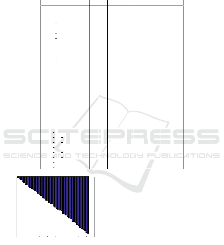
Table 1: The largest two Hankel singular values for modified COMPl
e
ib examples of generalized systems. The number j is
the index for which λ
j
is originally unstable; r is the number of significant Hankel singular values, that is, rank(R
o
R
c
). A
hyphen is used when there are no unstable eigenvalues.
Example n m p σ
1,2
j r
TL 256 2 2 1.018e+18 6.630e+17 - 41
HF2D1 3796 2 3 6.4334e-1 2.7337e-1 328 46
HF2D1 M316 316 2 3 3.5506e+0 6.2466e-1 29 40
HF2D1 M541 541 2 3 1.7852e+0 4.6071e-1 47 44
HF2D2 3796 2 3 2.3534e-1 8.5433e-2 328 47
HF2D2 M316 316 2 3 5.5555e-1 1.6910e-1 30 40
HF2D2 M541 541 2 3 5.6463e-1 1.5720e-1 47 42
HF2D3 4489 2 4 6.2163e-1 2.8049e-1 - 50
HF2D4 2025 2 4 1.7699e+1 3.1309e+0 - 44
HF2D5 4489 2 4 2.9820e+1 1.8711e+1 1 53
HF2D5 M289 289 2 4 3.0656e+0 2.1297e+0 4 41
HF2D5 M529 529 2 4 6.3719e+0 4.2424e+0 4 43
HF2D6 2025 2 4 8.0719e+0 5.3872e+0 9 46
HF2D6 M289 289 2 4 1.3787e+0 7.6935e-1 1 37
HF2D6 M529 529 2 4 4.1366e+0 2.6703e+0 1 41
HF2D7 4489 2 4 4.2784e+1 1.7350e+1 2 51
HF2D8 2025 2 4 8.9382e+0 3.6434e+0 9 46
HF2D10 5 2 3 1.9855e+0 3.8523e-1 3 5
HF2D11 5 2 3 1.1360e+0 1.4687e-1 3 5
HF2D12 5 2 4 6.3154e-1 2.4018e-1 - 5
HF2D13 5 2 4 1.7742e+1 3.3692e+0 - 5
HF2D14 5 2 4 2.8355e+1 1.0403e+1 2 5
HF2D15 5 2 4 7.9188e+0 3.4392e+0 2 5
HF2D16 5 2 4 4.3374e+1 1.5587e+1 2 5
HF2D17 5 2 4 8.9934e+0 3.9228e+0 2 5
HF2D IS1 4489 2 4 3.8087e+0 1.2708e+0 4 51
HF2D IS1 M361 361 2 4 2.9901e+0 1.3285e+0 1 41
HF2D IS1 M529 529 2 4 1.0183e+0 8.3036e-1 4 43
HF2D IS2 4489 2 4 3.4372e-1 2.2463e-1 9 49
HF2D IS2 M361 361 2 4 5.3589e-1 3.4371e-1 1 39
HF2D IS2 M529 529 2 4 4.6915e-1 3.0184e-1 1 42
HF2D IS5 5 2 4 1.6869e+0 3.3007e-1 2 5
HF2D IS6 5 2 4 3.2556e-1 6.2128e-2 2 5
0 5 10 15 20 25 30 35 40 45 50
i
-30
-25
-20
-15
-10
-5
0
ln(σ
i
)
Hankel singular values for COMPl
e
ib example HF2D1
Figure 2: Significant Hankel singular values of the modified
example HF2D1 from the COMPl
e
ib collection.
kel singular values for the larger system HF2D1, of or-
der 3796, modified similarly.
Table 1 shows the first two Hankel singular values
σ
1,2
for all 33 (modified) COMPl
e
ib real examples.
The number j is the index for which λ
j
is originally
unstable; r is the number of significant Hankel singu-
lar values, that is, rank(R
o
R
c
). A hyphen is used when
there are no unstable eigenvalues; this happened for
the five examples mentioned above.
The maximum total CPU execution time was of
46.46 minutes, for example HF2D5, with n = 4489,
m = 2, and p = 4. The most time consuming step is
the reduction to the RSF using the QZ algorithm. The
ratios between the timing values needed by this algo-
rithm and the solution of the two reduced equations
vary in the range (1.05, 3.35) and the mean value of
these ratios is 2.34. The ratios are larger for higher or-
der examples. Similarly, the ratios between the timing
values needed by QZ and the computation of the sin-
gular values vary in the range (14, 72) and the mean
value is 34.19. The total CPU time for each system of
order at most 541 was less than 3.16 seconds. Sim-
ilarly, each system of order 2025 needed less than
224 seconds. Other solvers would need by about 1.7
times more CPU time for each example, since the
computation of GSF should be done twice.
ICINCO 2022 - 19th International Conference on Informatics in Control, Automation and Robotics
136

All 33 examples have also been modified to obtain
and solve complex Lyapunov equations. However, 18
COMPl
e
ib examples have real eigenvalues only. For
these systems, the qz function returns real matrices
e
A
and
e
E. To get a complex dynamic system, the ma-
trix
e
A has been modified by adding ı|λ
j
|/ε
1/2
to
e
a
j j
,
where j is the index of the real eigenvalue with the
minimum modulus, and ε ≈ 2.22 · 10
−16
. The first
two largest singular values were the same as in Ta-
ble 1, except for HF2D1, HF2D2, HF2D12, and HF2D13,
for which they were somewhat larger.
7 CONCLUSIONS
New numerically attractive algorithms for solving sta-
ble generalized complex Lyapunov equations for both
continuous- and discrete-time systems is presented.
Two equations with the matrices A, E, and A
H
, E
H
,
respectively, can be solved using a single computa-
tion of the generalized Schur form. This is useful,
for instance, when finding the Hankel singular val-
ues of linear generalized dynamical systems. New
computational formulas are derived, and related nu-
merical issues are highlighted. The numerical re-
sults for a big set of examples, some of large order,
based on the COMPl
e
ib collection, illustrate the per-
formance of the software implementation. The CPU
computing time for finding the Hankel singular values
can be with 70% smaller than for other approaches.
Moreover, new scaling strategies allow to solve badly
scaled problems for which other implementations
would fail. The proposed solver is currently incor-
porated in SLICOT Library and MATLAB.
REFERENCES
Anderson, E., Bai, Z., Bischof, C., Blackford, S., Demmel,
J., Dongarra, J., Du Croz, J., Greenbaum, A., Ham-
marling, S., McKenney, A., and Sorensen, D. (1999).
LAPACK Users’ Guide: Third Edition. Software · En-
vironments · Tools. SIAM, Philadelphia, MA.
Bartels, R. H. and Stewart, G. W. (1972). Algorithm 432:
Solution of the matrix equation AX + XB = C. Comm.
ACM, 15(9):820–826.
Benner, P., Mehrmann, V., Sima, V., Van Huffel, S., and
Varga, A. (1999). SLICOT — A subroutine library in
systems and control theory. In Datta, B. N. (ed), Ap-
plied and Computational Control, Signals, and Cir-
cuits, vol. 1, pp. 499–539. Birkh
¨
auser, Boston, MA.
Benner, P. and Werner, S. W. R. (2020). Frequency-
and time-limited balanced truncation for large-scale
second-order systems. pp. 1–30. [Online]. Available:
https://arxiv.org/abs/2001.06185v1.
Bini, D. A., Iannazzo, B., and Meini, B. (2012). Numeri-
cal Solution of Algebraic Riccati Equations. SIAM,
Philadelphia, MA.
Cao, X., Benner, P., Duff, I. P., and Schilders, W. (2020).
Model order reduction for bilinear control systems
with inhomogeneous initial conditions. Int. J. Con-
trol, 1–10.
Dongarra, J. J., Du Croz, J., Duff, I. S., and Hammarling, S.
(1990). Algorithm 679: A set of Level 3 Basic Lin-
ear Algebra Subprograms. ACM Trans. Math. Softw.,
16(1):1–17, 18–28.
Golub, G. H. and Van Loan, C. F. (2013). Matrix Computa-
tions. The Johns Hopkins University Press, Baltimore,
MD, fourth edition.
Hammarling, S. J. (1982). Numerical solution of the stable,
non-negative definite Lyapunov equation. IMA J. Nu-
mer. Anal., 2(3):303–323.
Lancaster, P. and Rodman, L. (1995). The Algebraic Riccati
Equation. Oxford University Press, Oxford.
Leibfritz, F. and Lipinski, W. (2003). Description of the
benchmark examples in COMPl
e
ib. Tech. report, Dep.
of Mathematics, University of Trier, Germany.
MathWorks
®
(2015). Control System Toolbox
™
. The Math-
Works, Inc., Natick, MA.
Mehrmann, V. (1991). The Autonomous Linear Quadratic
Control Problem. Theory and Numerical Solution.
Springer-Verlag, Berlin.
Penzl, T. (1998). Numerical solution of generalized Lya-
punov equations. Advances in Comp. Math., 8:33–48.
Sima, V. (1996). Algorithms for Linear-Quadratic Opti-
mization. Marcel Dekker, Inc., New York.
Sima, V. (2019). Comparative performance evaluation of
an accuracy-enhancing Lyapunov solver. Information,
Special Issue ICSTCC 2018: Advances in Control and
Computers, 10(6 215). 22 pages.
Simoncini, V. (2016). Computational methods for linear
matrix equations. SIAM Rev., 58(3):377–441.
Stykel, T. (2002). Numerical solution and perturbation the-
ory for generalized Lyapunov equations. Lin. Alg.
Appl., 349(5):155–185.
Stykel, T. (2004). Gramian based model reduction for de-
scriptor systems. Math. Control Signals Syst., 16:297–
319.
Van Huffel, S., Sima, V., Varga, A., Hammarling, S., and
Delebecque, F. (2004). High-performance numeri-
cal software for control. IEEE Control Syst. Mag.,
24(1):60–76.
Varga, A. (2017). Solving Fault Diagnosis Problems: Lin-
ear Synthesis Techniques. Springer, Berlin.
Yang, S., Birk, W., and Cao, Y. (2020). A new controllabil-
ity index based on Hankel singular value. In Preprints
of the 21st IFAC World Congress (Virtual), pp. 4736–
4741, Berlin, Germany.
Solving Stable Generalized Lyapunov Equations for Hankel Singular Values Computation
137