
Comparison of SVM-based Feature Selection Method for Biological
Omics Dataset
Xiao Gao
a
Xi’an University of Posts & Telecommunications, Xi 'an, Shaanxi Province, China
Keywords: Cancer Classification, Feature Selection, Support Vector Machines, Recursive Feature Elimination.
Abstract: With the development of omics technology, more and more data will be generated in cancer research.
Machine learning methods have become the main method of analysing these data. Omics data have the
characteristics of the large number of features and small samples, but features are redundant to some extent
for analysis. We can use the feature selection method to remove these redundant features. In this paper, we
compare two SVM-based feature selection methods to complete the task of feature selection. We evaluate the
performance of these two methods on three omics datasets, and the results showed that the SVM-RFE method
performed better than the pure SVM method on these cancer datasets.
1 INTRODUCTION
Genomics and other related omics technologies have
been widely adopted to obtain new insights into the
pathogenesis of cancer patients. Machine learning is
a commonly used method to analyze these data, but
omics datasets have a large amount of repetitive and
strongly correlated feature (Karahalil 2016).
Redundant features affect the efficiency and accuracy
of machine learning models (Bhola and Singh 2018).
Therefore, we need feature selection technology to
process these datasets to improve the processing
efficiency and performance of our machine learning
model (Golub, Slonim, 1999).
Feature selection methods have many categories,
such as penalty-based method, tree-based method and
recursive feature elimination method and so on. The
penalty-based feature selection can automatically set
the small estimation coefficient to zero to reduce the
complexity of the model (Wang. Zhou. Wu. Chen.
Fan 2020). When we use tree-based models for
feature selection, after training any tree model, you
can access the feature importance attribute that ranks
features to complete the feature selection process
(Jotheeswaran, Koteeswaran 2015). Recursive
feature elimination (RFE) method is a very popular
and efficient feature selection method, which is
suitable for prediction models with feature weight as
a
https://orcid.org/0000-0003-1520-8704
model fitting result. The RFE algorithm obtains the
optimal combination of variables to maximize the
model performance by removing features recursively
(GUYON, WESTON, BARNHILL 2002). The
process of feature selection using recursive feature
elimination is as follows: Firstly, all feature variables
are used to train the model. Secondly, one of the worst
features is removed each time according to the
performance of the feature on the model. Thirdly, the
second step is recursively repeated until the number
of remaining features reaches the required number of
features.
There are many common feature selection
methods that can be combined with RFE
methodology for feature selection, such as support
vector machine (SVM) or random forest (RF). Boser
et al. proposed advanced SVM classification
algorithms in 1992 (Boser 1992, Vapnik 1998).
Moreover, Mukherjee et al. proposed SVM feature
selection method (Weston, Mukherjee, Chapelle,
Pontil, Vapnik 2001). SVM classifies samples by
finding a hyperplane that maximizes the distance
between classes in training data. The method of
feature selection using SVM is ranking the
importance of feature through the coefficients
attribute provided by SVM. When SVM-RFE is used
for feature selection, the features are evaluated
according to the performance of each feature on the
Gao, X.
Comparison of SVM-based Feature Selection Method for Biological Omics Dataset.
DOI: 10.5220/0011247400003443
In Proceedings of the 4th International Conference on Biomedical Engineering and Bioinformatics (ICBEB 2022), pages 595-600
ISBN: 978-989-758-595-1
Copyright
c
2022 by SCITEPRESS – Science and Technology Publications, Lda. All rights reserved
595

model, and then those less important features are
recursively deleted until the remaining number of
features meets our requirements (Meng, Yang 2008).
We can also improve time efficiency by removing
multiple features at a time, but it may lead to a decline
in model performance (Tang, Zhang, Huang 2007).
Random Forest was formally proposed by Leo
Breiman et al in 2001. The Random Forest feature
selection method (Genuer, Poggi, Tuleau-Malot
2016) is to access the feature importance attribute
after completing the random forest classifier fitting
and rank the features according to the importance.
Similarly, RF-RFE adopts an identical idea for the
procedure of RFE as SVM-RFE.
In this paper, we want to compare the
performance of SVM and SVM-RFE feature
selection methods on the omics dataset. Therefore,
we use these two feature selection methods to select
features on three cancer datasets, and the feature
selection performance is evaluated on Logistic
regression (LR) and random forest (RF) models.
The rest part of this article is as follows: Section
Ⅱ presents the theory of support vector machine and
recursive feature elimination. Section Ⅲ presents the
results on different cancer datasets using two feature
selection methods. In addition, we also studied the
influence of SVM-RFE each iteration to eliminate
different number of features on the model. Section Ⅳ
concludes our work and proposes future directions.
2 METHOD
2.1 Datasets
We used the cancer data set from TCGA database
(TCGA Network 2012). The TCGA database is a
project jointly supervised by the National Cancer
Institute and the National Human Genome Research
Institute a very comprehensive cancer genetic data.
In this paper, we used the miRNA datasets from
three cancer types in TCGA to compare the
performance of SVM and SVM-RFE feature
selection methods, namely thyroid cancer (THCA),
glioma (GBMLGG) and lung squamous cell
carcinoma (LUSC). The total number of THCA
patients is 569, including 510 tumor samples and 59
normal samples. The total number of GBMLGG
patients is 529, including 487 tumor samples and 42
normal samples. The total number of LUSC patients
is 387, including 342 tumor samples and 45 normal
samples. In addition, we preprocessed the dataset by
deleting all genes with zero median in all samples, as
shown in table 1.
Table 1: The number of features in datasets before and after
preprocessing.
Dataset Name
Before
p
rocessin
g
After
p
rocessin
g
THCA 1046 898
GBMLGG 1046 856
LUSC 1046 886
2.2 Feature Selection Method
2.2.1 Support Vector Machine (SVM)-
Based Feature Selection
Given training sample set D, to classify training set
sample D= {(x
1
, y
1
), (x
2
, y
2
), ..., (x
m
, y
m
)}, y
i
∈{-1,
+1}, we need to find a partition hyperplane in the
sample space based on the training set D. In the
sample space, the partition hyperplane can be
described by the following linear equation:
ω
T
x + b = 0 (1)
where ω is a normal vector, which determines the
direction of the hyperplane b is the displacement
term, which determines the distance between the
hyperplane and the origin. The partition hyperplane
can be determined by normal vector w and
displacement b. The distance from any point in the
sample to the hyperplane ( ω, b) can be expressed as:
𝑟=
‖
‖
(2)
If the hyperplane (𝜔, b) can correctly classify the
training samples, for (x
i
, y
i
) ∈D, if y
i
= + 1,ω
T
x
i
+ b
> 0, if y
i
= − 1, ω
T
x
i
+ b < 0:
𝜔
𝑥
+𝑏≥+1,𝑦
=+1
𝜔
𝑥
+𝑏≤−1,𝑦
=−1
(3)
As shown in the following figure 1, several training
samples points closest to the hyperplane make the
equality of Equation (3) hold, which are called
support vectors. The sum of the distances between
these two heterogeneous support vectors to the
hyperplane can be represented by formula (4), which
is called interval.
𝜸=
𝟐
‖
𝝎
‖
(4)
Figure 1: Support vector and interval.
ICBEB 2022 - The International Conference on Biomedical Engineering and Bioinformatics
596

Only support vectors work when deciding to
separate hyperplane, while other instances do not. If
the mobile support vector will change the solution;
but if you move other instance points outside the
margin, or even remove them, the points will not
change. Since support vector plays a decisive role in
determining hyperplane, this model is called support
vector machine. The number of support vectors is
generally small, so the support vector machine is
determined by a small number of important samples
(Drucker, Burgers, Kaufman, et al 1996).
Finding the appropriate ω and b such that 𝛾 is
the maximum partition hyperplane with the
maximum interval, that is, satisfying:
𝑚𝑖𝑛
1
2
‖
𝜔
‖
𝑠.𝑡. 𝑦
(𝜔
𝑥
+𝑏)≥1,𝑖 = 1, 2, …, m (5)
To sum up, there is the following linear separable
support vector machine learning algorithm -
maximum margin method
Algorithm: Linear separable support vector
machine learning algorithm
Input: Linear dataset = D= {(x
1
, y
1
), (x
2
, y
2
), ..., (x
m
, y
m
)}, y
i
∈{-1, +1}.
Output: Maximum separation hyperplane and
classification decision function.
When we use SVM for feature selection, we use
the weight of SVM classifier to generate feature
ranking. Linear SVM will provide the weight of each
feature after classification as the basis for feature
ranking.
Maximum separation hyperplane of linear
separable training dataset exists and unique.
Proof Existence:
Since the training data set is linearly separable, (5)
in the maximum interval method must have a feasible
solution, and because the objective function has a
lower bound, (5) must have a solution, denoted by (𝜔,
b). Since there are both positive and negative points
in the training data set, (𝜔, b) = (0, b) is not the
optimal feasible solution, so the optimal solution ( 𝜔,
b) must satisfy 𝜔 * / = 0. From this, we can know
the existence of separating hyperplane.
Proof Uniqueness:
When we use SVM for feature selection, we use
the weight of SVM classifier to generate feature
ranking. Linear SVM will provide the weight of each
feature after classification as the basis for feature
ranking
Firstly, the uniqueness of w * in the solution of
optimization problem (5) is proved. Suppose problem
(5) has two optimal solutions ( 𝜔
1
*, b
1
*) and ( 𝜔
2
*, b
2
*). Obviously | | 𝜔 * 1 | | = | | 𝜔 * 2 | | = c,
where c is a constant. Let 𝜔=
∗
∗
, 𝑏=
∗
∗
,it is
easy to know that ( 𝜔, b) is the feasible solution of
problem (5), so c ≤
‖
𝜔
‖
≤
𝜔
∗+
𝑤
∗
=
𝐶,the above equation indicates that the unequal sign
in the equation can be changed into an equal sign,
That is
‖
𝜔
‖
=
𝜔
∗
+
𝜔
∗
, Thus 𝜔
∗
=𝜆𝜔
∗
,
|
𝜆
|
=1.if 𝜆 = -1, then 𝜔 = 0, ( 𝜔, b ) is not a
feasible solution to problem ( 5 ). So 𝜆 = 1, that
is𝜔
∗
=𝜔
∗
. Thus, the two optimal solutions ( 𝜔
∗
,
𝑏
∗
) and ( 𝜔
∗
, 𝑏
∗
) can be written as (𝜔
∗
, 𝑏
∗
) and
(𝜔
∗
, 𝑏
∗
), respectively. It is further proved that 𝑏
∗
=
𝑏
∗
. Let 𝑥
, 𝑥
and set {
𝑥
|
𝑦
=+1
} correspond
to the points where ( 𝜔
∗
, 𝑏
∗
) and ( 𝜔
∗
, 𝑏
∗
) make
the inequality of the problem hold, respectively,
corresponding to 𝑥
and 𝑥
,in set
𝑥
|
𝑦
=−1
,then from 𝑏
∗
=−
(
𝜔
∗
⋅𝑥
+𝜔
∗
⋅𝑥
)
, 𝑏
∗
=
−
(
𝜔
∗
⋅𝑥
+𝜔
∗
⋅𝑥
)
, 𝑏
∗
− 𝑏
∗
=−
𝑤
∗
⋅
(
𝑥
−
𝑥
)
+𝜔
∗
⋅
(
𝑥
−𝑥
)
is obtained. Because 𝜔
∗
⋅
𝑥
+𝑏
∗
≥1=𝜔
∗
⋅𝑥
+𝑏
∗
, 𝜔
∗
⋅𝑥
+𝑏
∗
≥1=
𝜔
∗
⋅𝑥
+𝑏
∗
,so 𝑤
∗
⋅
(
𝑥
−𝑥
)
=0 is the same as
𝑤
∗
⋅
(
𝑥
−𝑥
)
=0. Therefore, 𝑏
∗
− 𝑏
∗
= 0 can be
seen from 𝜔
∗
= 𝜔
∗
that the two optimal solutions
( 𝜔
∗
, 𝑏
∗
) and ( 𝜔
∗
, 𝑏
∗
) are the same, and the
uniqueness of the solution is proved. From the
uniqueness of solution of formula (5), it is concluded
that the separated hyperplane is unique (C. Platt
1999).
2.2.2 Support Vector Machine-Recursive
Feature Elimination (SVM-RFE)
Firstly, in each round of training process, all features
are selected for training, and then the hyperplane 𝜔
T
x + b = 0 is obtained. If there are n features, then
SVM-RFE will select the feature corresponding to the
sequence number i with the least square value of the
component in w, and delete it. In the second class, the
number of features remaining n-1, continue to use
these n-1 features and output values to train SVM.
Similarly, continue to remove the features
corresponding to the minimum square value of the
component in w. In this way, until the remaining
number of features meet our requirements.
In order to better evaluate the performance
fluctuation in the feature selection process, it is
necessary to add a layer of resampling process to the
outer layer of the above algorithm. This experiment
uses K-fold cross validation.
The overall process of the algorithm is as follows:
algorith
m
1.For each resamplin
g
iteration
1.1 The most important feature variable S {i}
b
efore extraction
Comparison of SVM-based Feature Selection Method for Biological Omics Dataset
597
1.2 Training model based on new dataset
1.3 Validation Set Assessment Model
1.4 Split the training set into new training set
and verification set
1.5 Training model with new training set and
all characteristic variables
1.6 Evaluation model using validation sets
1.7 Calculate and sort the importance of all
feature variables
1.8 For each variable subset S {i},i = 1... S :
2. Determining an appropriate number of
characteristic variables
3. Estimate the set of characteristic variables
for final model construction
4. Selecting the optimal variable set and
b
uilding the final model with all training sets
2.3 Evaluation of Feature Selection
Methods
This section must be in two columns.
Each column must be 7,5-centimeter wide with a
column spacing of 0,8-centimeter.
The section text must be set to 10-point, justified
and linespace single.
Section, subsection and sub subsection first
paragraph should not have the first line indent, other
paragraphs should have a first line indent of 0,5-
centimeter.
In order to compare the performance of
SVM and SVM-RFE feature selection methods, the
two methods are used to select the same number of
features on three datasets, and then LR and RF
classifiers and K-fold cross validation are used. F1
and AUC are used as metrics of this method. For
SVM-RFE eliminating the influence of different
number of features each time on the model, we set up
three different iterative elimination features to
compare the performance of the model.
Specially, the linear kernel SVM is used in our
experiment, and the penalty coefficient C in SVM is
set to 1, so that it has good generalization ability. In
the SVM-RFE method, one feature is deleted
recursively each time to maximize the model
performance.
The metrics we use relate to True Positive (TP),
True Negative (TN), False Positive (FP), and False
Negative (FN) are involved. The first metrics is F1,
F1 combines Precision and Recall, and its evaluation
is more balanced.
F1 =
∗∗
(6)
The second evaluation index is roc-auc, roc curve
is the relationship between FPR and TPR. By drawing
the ROC curve, we can observe the performance of
the model. The better the performance of the model,
the closer the ROC curve is to the solid shallow gray
line in the upper left corner of Figure 2.
The x-axis is false positive rate (FPR):
FPR=
(7)
The y-axis is true positive rate (TPR):
TPR=
(8)
AUC is the area covered by the ROC curve.
Obviously, the larger AUC is, the better the classifier
classification effect is.
3 RESULTS
3.1 The Number of Features
Eliminated in Each Iteration
Affects Feature Selection
Performance
For the mutual benefit and protection of Authors and
Publishers, it is necessary that Authors provide
formal written Consent to Publish and Transfer of
Copyright before publication of the Book. The signed
Consent ensures that the publisher has the Author’s
authorization to publish the Contribution.
The copyright form is located on the authors’
reserved area.
The form should be completed and signed by one
author on behalf of all the other authors.
To investigate whether the number of features
removed in each iteration affects the performance of
the SVM-RFE feature selection method, we used
SVM-RFE to remove a different number of features
in each iteration on three cancer datasets. Finally, LR
and RF classifiers were used to compare the feature
selection results.
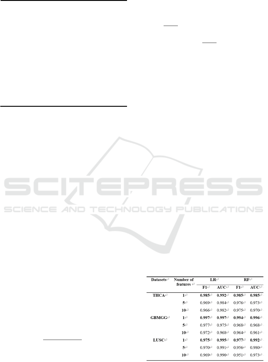
Table 2: Eliminating the performance impact of different
number of features each time.
ICBEB 2022 - The International Conference on Biomedical Engineering and Bioinformatics
598
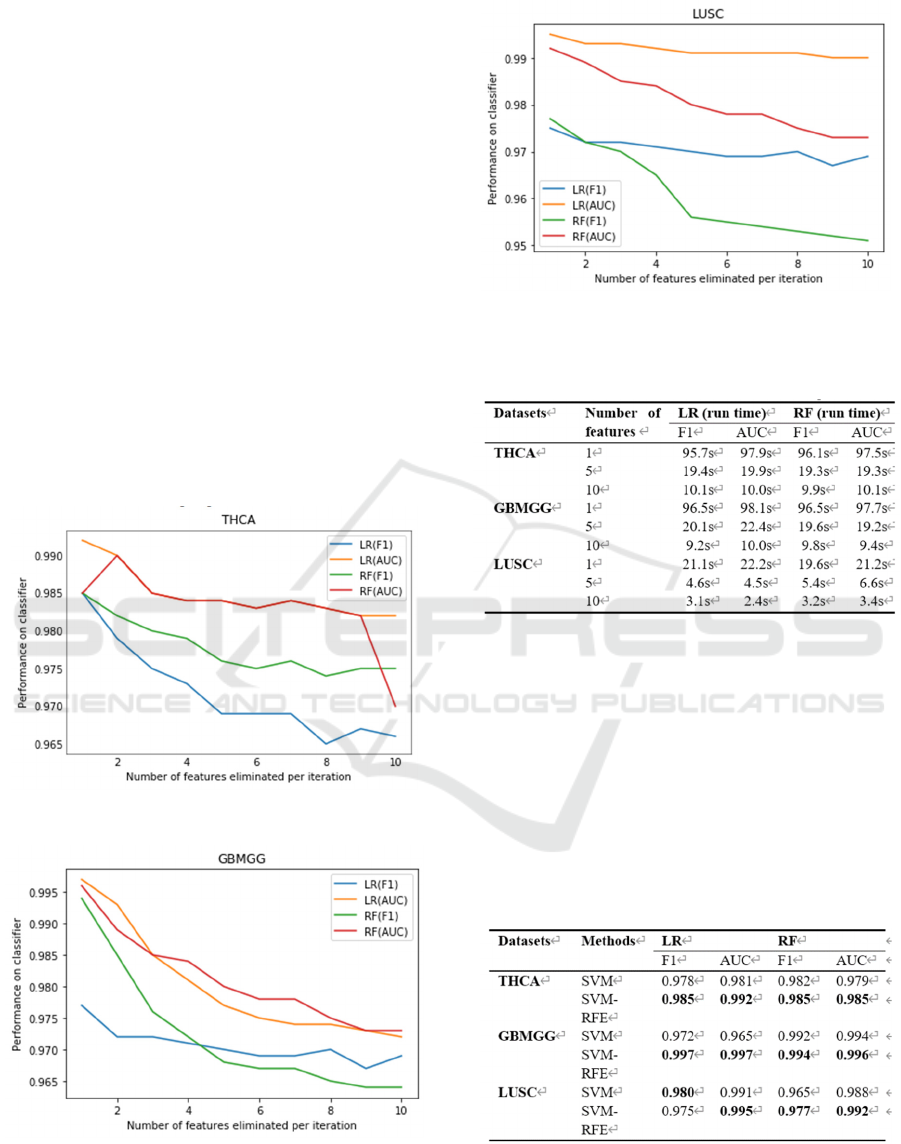
TABLE 2 shows the performance of SVM-RFE
in deleting the different number of features in each
iteration. In the SVM-RFE feature selection method,
one or more features can be eliminated each time, and
it can be seen from the table that the model performs
best when one feature is eliminated each iteration. We
speculate that when a set of features consisting of
multiple features is removed each time, we take the
overall importance of a set of features as the
evaluation criterion. The deficiency of this is that
although the other set of relatively insignificant
features is removed, the importance of each feature
within the relatively important set of features cannot
be judged. It is possible that there is a group of
features with high overall importance, but some
unimportant features in the group are not removed.
Therefore, eliminating multiple features each time
may cause a certain degree of performance
degradation.
The relationship between the number of features
eliminated per RFE iteration and performance is
shown in the following figure.
Figure 2: On the THCA dataset.
Figure 3: On the GBMGG dataset.
Figure 4: On the LUSC dataset.
Table 3: The influence of eliminating different number of
features each time on feature selection time consumption.
TABLE 3 shows the time cost for SVM-RFE to
delete different number of features each iteration, the
more features are eliminated each iteration, the less
time is spent on feature selection. TABLE4.
Evaluating feature selection methods using LR and
RF models
3.2 Comparison between SVM and
SVM-RFE Feature Selection
Methods
Table 4: Evaluating feature selection methods using LR and
RF models.
Table 4 shows performance on LR and RF classifiers
after selecting 20 features from three TCGA cancer
datasets using SVM and SVM-RFE methods. The
results show that the SVM-RFE feature selection
method achieves better performance than the SVM
Comparison of SVM-based Feature Selection Method for Biological Omics Dataset
599

feature selection method on all these three datasets.
For example, in THCA dataset, SVM-RFE method is
about 0.7 % higher than SVM, while in GBMGG
dataset, SVM-RFE method is about 0.2 % to 2 %
higher than SVM. On LUSC dataset, the F1 score of
SVM-RFE method is slightly lower than SVM only
when using LR classifier, and the other scores are
higher than SVM
4 CONCLUSIONS
In this paper, two feature selection methods based on
SVM are compared, and this method is applied to
three different TCGA cancer datasets to verify and
compare their performance on two classifiers.
Finally, it is concluded that the comprehensive
performance of the SVM-RFE feature selection
method is better than that of the SVM feature
selection method.
In addition, we did a further experiment on the
performance of SVM-RFE, by eliminating a different
number of features to explore the impact of SVM-
RFE each iteration on the model performance. The
conclusion is that when we use SVM-RFE, the model
performs best when one feature is removed in each
iteration, but it takes a long time. Eliminating
multiple features in each iteration improves the time
efficiency of the model, but reduces its performance.
This experiment is of great significance to the study
of cancer, further verifying the feasibility of machine
learning in cancer data analysis, helping doctors and
researchers to reduce the pressure of analyzing cancer
data, and helping predict the patient's condition.
Suggestions for further work: Analyze whether the
patient's condition is serious by judging whether the
patient is in the primary state of cancer or the
metastatic state of cancer lesions. Divide tumors into
types and adopt different treatment options to
improve the patient's 5-year survival rate.
ACKNOWLEDGEMENTS
Throughout the writing of this dissertation, I have
received a great deal of support and assistance. I
would like to thank my parents for their wise counsel
and sympathetic ear. You are always there for me. I
could not have completed this dissertation without the
support of my friends, who provided stimulating
discussions as well as happy distractions to rest my
mind outside of my research.
REFERENCES
Comparison of Penalty-based Feature Selection Approach
on High Throughput Biological Data. N Wang.W
Zhou.J Wu.S Chen.Z Fan(2020)
Comprehensive molecular portraits of human breast
tumours, TCGA Network (2012)
Decision tree based feature selection and multilayer
perceptron forsentiment analysis. J Jotheeswaran.S
Koteeswaran (2015)
Development of Two-Stage SVM-RFE Gene Selection
Strategy for Microarray Expression Data Analysis, Yu
chun Tang, Yan-Qing Zhang, and Zhen Huang (2007).
Feature selection for support vector machines. J Weston, S
Mukherjee, O Chapelle, M Pontil, V Vapnik(2001)
ISABELLE GUYON, JASON WESTON, STEPHEN
BARNHILL Gene Selection for Cancer Classification
using Support Vector Machines, AT&T Labs, Red
Bank, New Jersey, USA, (2002,7-14).
Molecular Classification of Cancer: Class Discovery and
Class Prediction by Gene Expression Monitoring.T. R.
GoLub, 12*t D. K. SLonim,1t P. Tamayo,' C.
Huard,'M. Gaasenbeek,l J. P. Mesirov,1 H. CoUler,1
M. L. Loh,2 J. R. Downing,3 M. A. Caligiuri,4 C. D.
Bloomfield,4 E. S. Lander (1999)
Multiclass SVM-RFE for product form feature selection.
Meng-Dar Shieh *, Chih-Chieh Yang (2002)
Overview of Systems Biology and Omics Technologies.
Bensu Karahalil (2016).
Platt J C. Fast train of support vector machines using
sequential minimal optimization (1999).
Support Vector Machines, Boser, (1992); Vapnik, (1998)
Support vector regression machines. In: Advances in
Neural Information Processing Systems 9, Drucker J,
Burgers C J C, Kaufman L,er al., NIPS 1996. MIT
Press, 155-161
Variable selection using Random Forests. Robin Genuer,
Jean-Michel Poggi, Christine Tuleau-Malot (2016).
WA. Bhola and S. Singh (2018), “Gene selection using high
dimensional gene expression data: An appraisal.
ICBEB 2022 - The International Conference on Biomedical Engineering and Bioinformatics
600
