Control-relevant Model Selection for Multiple-mass Systems

∗

Mathias Tantau

1 a

, Torben Jonsky

2 b

, Zygimantas Ziaukas

1 c

and Hans-Georg Jacob

1 d

Institute of Mechatronic Systems, Leibniz University Hannover, An der Universit

at 1, 30823 Garbsen, Germany

Lenze SE, Hans-Lenze-Str. 1, 31855 Aerzen, Germany

Keywords:

Control-relevant Model Selection, Model-based Control, Multiple-mass Systems, Non-parametric Models,

Modelless Simulation.

Abstract:

Physically motivated parametric models are the basis of several techniques related to control design. Industrial

model-based controller tuning methods include pole placement, symmetric optimum and damping optimum.

The challenge is that the resulting model-based controller is satisfactory only if the underlying model is ap-

propriate. Typically, a set of potential models is known a priori, but it is not known, which model should be

used. So, the critical question in model-based controller tuning is that of model selection. Existing approaches

for model selection are mostly based on maximizing accuracy, but there is no reason why the most accurate

model should also be the optimal model for control design. Given the overall aim to design a high-performance

controller, in this paper the best model is considered as the one that has the potential to give a model-based

controller the highest performance. The proposed method identiﬁes parametric candidate models for control

design. Then, a nonparametric model is used to predict the actual performance of the various controllers on

the real system. A validation with two industry-like testbeds shows success of the method.

1 INTRODUCTION

Physically motivated parametric models with inter-

pretable inner structure combine prior knowledge

with identiﬁcation measurements. These bright-grey

box models are the basis of several techniques related

to control design (Sch

utte, 2003), observers, feed-

forward and model-based fault diagnosis (Witczak

et al., 2002).

The advantages of deﬁning control parameters on

the basis of physically motivated models as opposed

to black-box models or completely model-free de-

signs include:

1. simplicity, transparency,

2. online adaptability to changing parameters and

model reference adaptive control (Khan et al.,

2013; Riva et al., 2016),

https://orcid.org/0000-0003-1195-7329

https://orcid.org/0000-0002-0512-1253

https://orcid.org/0000-0001-9161-0709

https://orcid.org/0000-0001-5605-9704

∗

This work was carried out as part of the research

project ”Automated Control Design based on (partly) au-

tomatically generated, Control-optimal Models” (FVA 665

IV), sponsored by the German Forschungsvereinigung

Antriebstechnik e.V. (FVA)

3. optimality, e.g. pole placement, settling time,

4. predictability of robustness to changing system

parameters,

5. low number of hyperparameters in the design, as

opposed to modern H

∞

control (Toscano and Ly-

onnet, 2009).

In the industrial ﬁeld of servo system control sev-

eral model-based methods are widely known, but nev-

ertheless model-less methods such as Ziegler-Nichols

are still used to set the control parameters in most

cases. A reason is that the selection of an appropri-

ate model among a set of known candidates is a major

difﬁculty and performance of model-based controllers

hinges critically on the suitabiliy of their models. For

example, it may not be known a priori if elasticities

in the structure should be considered or if they can be

neglected. An attempt to perform a model selection

including mulitple-mass systems, backlash and fric-

tion is delineated in (Sch

utte et al., 1997), but it is

not fully automatic. Models for control design tend

to be rather simple, including only a few parameters.

It is therefore important that the most dominant char-

acteristics are identiﬁed as such which would require

considerable effort and expert knowledge in practice

if this task was performed manually. Especially when

specialized systems such as stacker cranes, position-

Tantau, M., Jonsky, T., Ziaukas, Z. and Jacob, H.

Control-relevant Model Selection for Multiple-mass Systems.

DOI: 10.5220/0011231200003271

In Proceedings of the 19th International Conference on Informatics in Control, Automation and Robotics (ICINCO 2022), pages 605-615

ISBN: 978-989-758-585-2; ISSN: 2184-2809

605

ing systems and individual machine tools are commis-

sioned in small quantities, model development comes

at a comparatively high cost.

Methods for automatic model selection have been

described (Aguilar et al., 2001; Tantau et al., 2020;

Brun et al., 2001), which are mostly based on pre-

diction accuracy as a sole criterion for goodness of

the model, possibly in combination with parsimony

requirements. Commonly, several models are identi-

ﬁed and the one with the best ﬁt on a separate vali-

dation dataset is nominated as the optimal model. In-

stead of separate validation data information criteria

can be used (Chatﬁeld, 1995). For servo systems with

high quality actuators and sensors it can be expected

that these stochastic criteria result in overly complex

models, unlike the simple models known from control

design. This suggests that accuracy is not a suitable

model selection criterion in view of control design.

A control-relevant criterion for model selection

is required. In the ﬁeld of parameter identiﬁca-

tion control-relevant cost functions have been de-

ﬁned (identiﬁcation for control) (Van Den Hof and

Schrama, 1994; Hjalmarsson et al., 1996; Van den

Hof, 1997; Gevers, 2004; Jansson, 2004; Codrons,

2005; Saha et al., 2021). Mostly, the overall aim is

seen as to design a model-based controller with high

performance on the real system and accordingly the

optimal model is deﬁned as the one with lowest per-

formance degradation from model to real system or

good worst-case performance (among other require-

ments). The cost function considers a given controller

transfer function (Oomen et al., 2013) or if the con-

troller transfer function is not known yet at the stage

of identiﬁcation, not even approximately, the ν-gap

metric is used for identiﬁcation which allows to re-

place this knowledge by worst-case statements (Date

and Vinnicombe, 2004; Geng et al., 2015; Yang et al.,

2018).

One way to extend identiﬁcation for control to

model selection would be to use these control-relevant

cost functions also for selection of the best model.

This has been done in a few cases, see for example

(van Herpen et al., 2010; van Herpen et al., 2011;

Tacx et al., 2021; Tantau et al., 2022). This would

favour again the most accurate models, where accu-

racy is measured in a special, control-relevant way.

A slightly different approach is to also evaluate the

nominal performance that can be achieved with each

model, not only the performance degradation. This

has already been considered in these references. In

this sense the best model is the one with the poten-

tial to give a model-based controller the best perfor-

mance on the real system. With this reasoning, the

best model is not necessarily the most accurate one.

In this paper the idea of selecting the model that

gives a model-based controller the highest perfor-

mance is adopted, but the solution approach is very

different, adopted to physically motivated models and

common, industrial control design rules rather than

∞

-control. We propose to perform parameter identi-

ﬁcation for a couple of parametric models in a ﬁrst ex-

periment. Then, several commonly known controllers

are parametrized for each model. Finally, the differ-

ent resulting controller settings are validated on a non-

parametric model in order to predict their stability and

performance on the real system without actually car-

rying out hardware experiments, see below. The con-

troller with the best performance deﬁnes the optimal

model as the one that it is based on. Assuming that for

each model the most promising controllers are tested,

this procedure should output the model with potential

to give a model-based controller the highest perfor-

mance. What should facilitate applying this approach

in industry, is that it is close to well known and es-

tablished control design methods. The model selec-

tion strategy is similar to a manual model selection

but more systematic and it requires less hardware ex-

periments.

2 SET OF MODEL-BASED

CONTROLLERS

In this section several commonly used model-based

PI-controllers for speed control of electric motors

with coupled mechanics are introduced brieﬂy. They

will be considered in the model selection of Sec. 4.

Further details and derivations can be found in the

cited references. Nonlinear characteristics are left out

because the proposed method for model selection, see

Sec. 3, can only handle transfer function models. The

underlying transfer function models are identiﬁed in

a ﬁrst experiment as candidate models.

2.1 Symmetric Optimum for Systems

with Delay Time

If elasticities in the mechanics can be neglected and

the overall inertia of motor and load J

sum

is the only

parameter that describes the mechanics, a valid plant

model is given by:

G(s) =

sum

(1 + T

. (1)

accounts for the limited sampling frequency in the

current controller and the velocity measurement ﬁlter.

In this case the PI-speed controller can be tuned ac-

cording to the symmetric optimum in a way that the

ICINCO 2022 - 19th International Conference on Informatics in Control, Automation and Robotics

606

Figure 1: Chosen pole placement principles for 2-mass-

systems. Blue: identical damping, red: identical real part,

green: identical radius. When more than one principle is

possible, identical damping is preferred over identical real

part over identical radius.

zero-crossing frequency coincides with the maximum

phase (Tripathi et al., 2015):

sum

, T

= a

. (2)

a is a free parameter with the relation to the Lehr’

damping ratio D of the closed-loop poles a = 2D + 1.

a = 2 corresponds to optimal performance but a =

3 is more robust (Schr

oder, 2015). In the following

experiments a = 3 is chosen.

Alternatively, the symmetric optimum can be de-

signed for the ﬁrst mass only of an elastically cou-

pled system as a simple way to account for elasticity

and transition elements with unknown properties such

as belt drives and gear boxes. More advanced meth-

ods for mulitple mass system control design are given

next.

2.2 Pole Placement for 2-mass-systems

Zhang (Zhang and Furusho, 2000) argues that for the

two pole pairs of a controlled 2-mass-system there are

three reasonable pole placement objectives: identical

damping, identical real part and identical radius. De-

pending on the ratio of load inertia divided by motor

inertia R = J

and the damping speciﬁed for the

ﬁrst pole pair ζ

these objectives may be achievable

or not, see Fig. 1. In the ﬁgure a certain objective

is considered achievable only if the damping ratio re-

sulting for the second pole pair is 0.5 or more. For

details see (Zhang and Furusho, 2000).

2.3 Optimal Damping Design for 2- or

3-mass-systems

Another popular controller design method, that has

been used with 2-mass-systems, is the optimal damp-

ing design (Wertz and Schutte, 2000). It is based on

specifying double ratios. To obtain these the denomi-

nator polynomial of the closed control loop is written

in the form

P(s) = a

+ ··· + a

s + a

. (3)

Adjacent coefﬁcients have the ratios V

/(a

i−1

),i = 1 . ..n. The double ratios are de-

ﬁned as V

i−1

= a

i−2

i−1

,i = 2 . ..n, while

the reciprocal values are sometimes called stability

indices (Manabe, 1998). In (Manabe, 1998) it is

recommended to aim for D

n−1

= · ·· = D

= 0.5 and

= 0.4, as this gives the controlled system the

properties of low overshooting, short settling time

and a pole arrangement combining identical damping

and identical real part. The control parameters can be

chosen in fulﬁlment of these equations. If required,

another deﬁning equation can be generated by also

specifying the system time V

= a

n−1

(Schr

oder,

2015).

In the case of 2-mass-system speed control with

PI-controller the denominator polynomial has ﬁve co-

efﬁcients and three double ratios. Only the ﬁrst two

double ratios are speciﬁed to determine the two con-

trol parameters, because they are known to be more

important than the last double ratios (Sch

utte, 2003).

Out of the solutions one with positive real values is

chosen which may not always exist.

For 3-mass-systems ﬁve double ratios exist and

only two control parameters. Only the ﬁrst two damp-

ing ratios are deﬁned directly while the last three can

assume arbitrary values.

3 MODEL SELECTION

PROCEDURE

Having deﬁned the candidate models and controllers

in the preceding section this section explains the

model selection procedure, starting with an overview

followed by a more detailed description of certain

points.

3.1 Description of the Model Selection

Method

The procedure can be outlined as follows:

1. Parameter identiﬁcation for a set of physically

motivated candidate models based on a measured

frequency response function (FRF) of the system

2. Model-based control design / parametrization, as

described in Sec. 2. For each model all potential

controllers are parametrized.

Control-relevant Model Selection for Multiple-mass Systems

607

3. Veriﬁcation of all controllers via nonparametric

models, as described in this section. The model

corresponding to the best controller will be the

best model.

4. Hardware tests of the resulting controller settings.

The parameter identiﬁcation minimizes the sum of

squared errors between model and plant FRF over all

measured frequencies in the simplest case. The plant

FRF, which is needed for this step, should be mea-

sured in a way that artefacts from the closed control

loop are kept low, for example by inserting the excita-

tion at r

in Fig. 2, while the controller is disabled. In

the second step, if a certain controller cannot be pa-

rameterized for the given model parameters, e.g. be-

cause the control parameters would be complex, it is

left out.

In the third step the various controllers are tested

on a nonparametric model in order to predict their

stability and performance on the real system without

actually carrying out hardware experiments. It is as-

sumed that for each model the most promising con-

trollers are considered. Then, the best controller de-

ﬁnes its model as the one that can give a model-based

controller the highest performance.

Performance should not be measured in combina-

tion with the model that a certain controller is opti-

mized for, because this would be a trivial test; the

performance would be ideal mostly. Instead, condi-

tions should be close to performing veriﬁcation ex-

periments on the real hardware. This leads to the ap-

plication of complex, nonparametric models. Exam-

ples of nonparametric models are the impulse or step

response or the frequency response function (FRF).

Stability is checked by evaluating the Nyquist cri-

terion for the open loop consisting of plant FRF and

controller transfer function.

Furthermore it would be desirable to know the

step response so as to evaluate settling time, over-

shooting and integral criteria as performance mea-

sures. Time-domain signals are more intuitive for

many operators. The step response can be calcu-

lated from the system’s FRF, as explained in the next

section, so that a nonparametric model is available

for this kind of validation, too. Alternatively, time-

domain signals could be obtained from the convolu-

tion of the system’s impulse response (Risuleo, 2016).

Because of the linear nature of the transfer func-

tion nonlinear plant characteristics, e.g. friction,

backlash, and saturation cannot be considered explic-

itly and it is expectable that the methods fail if they

are dominant. Extensions to nonlinear models such

as long short-term memory networks would be con-

ceivable but the experimental effort for training seems

inappropriate for simple PI control design.

3.2 Step Response from

Frequency-domain Measurements

As an evaluation of the model-based controllers with

a nonparametric model step responses are calculated

numerically. Using the measured FRF of the sys-

tem together with the calculated transfer function

(tf) of the controller this is a question of converting

frequency-domain responses into a time-domain sig-

nals.

This could be done via inverse Laplace trans-

form by calculating the Bromwich inversion integral

(Grassmann, 2013):

f (t) = −

2πi

c+i∞

c−i∞

F(s)e

ds, (4)

in which c is a constant larger than the maximum real

part of the poles of the Laplace transform F(s). Meth-

ods for the numerical approximation of the integral

can be found for example in (Hosono, 1981; Abate

and Whitt, 2006; G

omez et al., 2007).

However, from the FRF the transfer function is

only known for c = 0. Setting c = 0 the Fourier trans-

form results (Grassmann, 2013):

f (t) =

2π

∞

−∞

F(iω)e

iωt

dω. (5)

Practically, it must be approximated via sum or trape-

zoidal integration method and only a ﬁnite maximal

frequency can be considered. Further simpliﬁcations

can be made if the time signal at negative times is not

of interest, which is usually the case for causal sys-

tems (Tan et al., 2017).

The restriction to c = 0 forbids to calculate the

time signal of transfer functions with nonnegative

poles, for example undamped resonating systems or

the s in the denominator introduced by the step excita-

tion. Put differently, the signal in time must decay. It

is therefore usually easiest to reconstruct the impulse

response at ﬁrst and to integrate it afterwards.

Another approach is to replace the step excitation

by a periodic, mean-free square wave, e.g. periodic

steps from −1 to 1 and from 1 to −1 and to assume

that the system has been exposed to this excitation for

a long time already. Now the system response h(t)

is periodic and can be calculated by means of Fourier

series expansion, see derivation in (Tan et al., 2017):

h(t) =

∞

∑

k=1(2)

{

F(ikω

)

}

sin(kω

t). ..

Im{F(ikω

)}cos(kω

t).

(6)

F(ikω

) refers to the system for which the step re-

sponses are of interest. In the context of controller

ICINCO 2022 - 19th International Conference on Informatics in Control, Automation and Robotics

608

validation F(ikω

) is a spectral line of the closed feed-

back loop of plant and controller. The 2 in brack-

ets means that every second frequency component is

skipped. Note that the frequency component 0 is not

evaluated, which in contrast to some other methods

also allows to calculate the system response of sys-

tems with one pole in the origin, but the calculated

system response is not quite correct in this case be-

cause initial conditions are neglected. These could

lead to an arbitrary offset on the output which is not

considered, instead h(t) is always centred around 0.

Apart from that the system should be stable.

Out of the step responses from −1 to 1 the step

responses from 0 to 1 or between two other con-

stants can be calculated by scaling the obtained re-

sults, as long as the (controlled) system has a limited

and known static gain: The output offset will be the

input offset times the static gain and the output ampli-

tude will be the input amplitude times the static gain.

This is related to the linearity of the considered sys-

tems, so an offset in the input will lead to a constant

offset of known height in the output after settling mo-

tions have decayed. For an integrator the condition of

a static gain is violated as the static gain is inﬁnite.

This method can be implemented efﬁciently with

the Matlab function ifft leading to short calculation

times.

Because in ﬁrst experiments the integration of the

impulse response showed to be inaccurate, in the fol-

lowing only the Fourier series method with square

wave excitation is used, the accuracy of which will be

demonstrated in Sec. 4. It is known that the conver-

sion from frequency-domain measurements to time-

domain signals is generally unstable and especially

high-frequency oscillations can be introduced by mi-

nor errors in the measured transfer function (Doetsch,

1985). So the accuracy of the step response recon-

struction will be pivotal in the remainder of the paper.

3.3 Calculation of the Closed-loop

System Response in

Frequency-domain

The Fourier transform of the closed-loop control sys-

tem, which is needed in (6), could be calculated from

the plant FRF P(iω) identiﬁed in open loop and the

known controller TF C

dest

(s) (SISO case):

cl,dest

(iω) =

P(iω)C

dest

(iω)

1 + P(iω)C

dest

(iω)

. (7)

For the setup in Fig. 2 this means that r

is used to

inject the excitation while C(iω) is set to zero.

However, calculating the closed loop in this way

would be inaccurate because the exact behaviour of

Figure 2: Control loop after (Van Den Hof and Schrama,

1994) with controller C(iω), plant P

(iω), output y, mea-

surement noise v and two possible excitations r

and r

the industrial drive C

dest

is not known in detail (ﬁlters,

resampling, time delay, etc.).

Instead, the closed loop is measured directly

with excitation at r

for a given, working controller

origin

(iω), which is ideally close to the controller

to be designed, for example the default setting pro-

vided by the manufacturer. Calling this measured

FRF G

cl,origin

(iω) the system’s FRF is extracted via:

P(iω) =

cl,origin

(iω)

origin

(iω)(1 − G

cl,origin

(iω))

. (8)

Then the closed loop FRF is calculated for the to be

designed controller via (7), using P(iω) from (8). In

this way the closed-loop FRF is still relatively accu-

rate, even if the true controller transfer functions are

not known exactly, at least when C

origin

and C

dest

are

close. If they are even identical, insufﬁcient knowl-

edge about ﬁlters, resampling, time delay, etc will not

lead to any errors. P(iω) contains some of these dis-

tortions and is therefore not useful if one is interested

in the FRF of the system alone.

This approach is in agreement with the claim of

’identiﬁcation for control’, which dictate to measure

a system or to identify a model in a way that is close

to the intended use of the model, resp. measurement.

For example, if a model is needed for closed-loop

predictions it should also be measured in closed loop

(Gevers and Ljung, 1986; Van Den Hof and Schrama,

1994; Hjalmarsson et al., 1996; Van den Hof, 1997;

Vinnicombe, 2001).

If at low frequencies G

cl,origin

(iω) is close to one

or exactly one, then (8) cannot be calculated directly.

In this case it is sufﬁcient to note that P(iω) is a very

high number.

4 EXPERIMENTAL RESULTS

This section is intended to demonstrate the model

selection procedure and the calculation of step re-

sponses from controller transfer function and non-

parametric system model.

Control-relevant Model Selection for Multiple-mass Systems

609

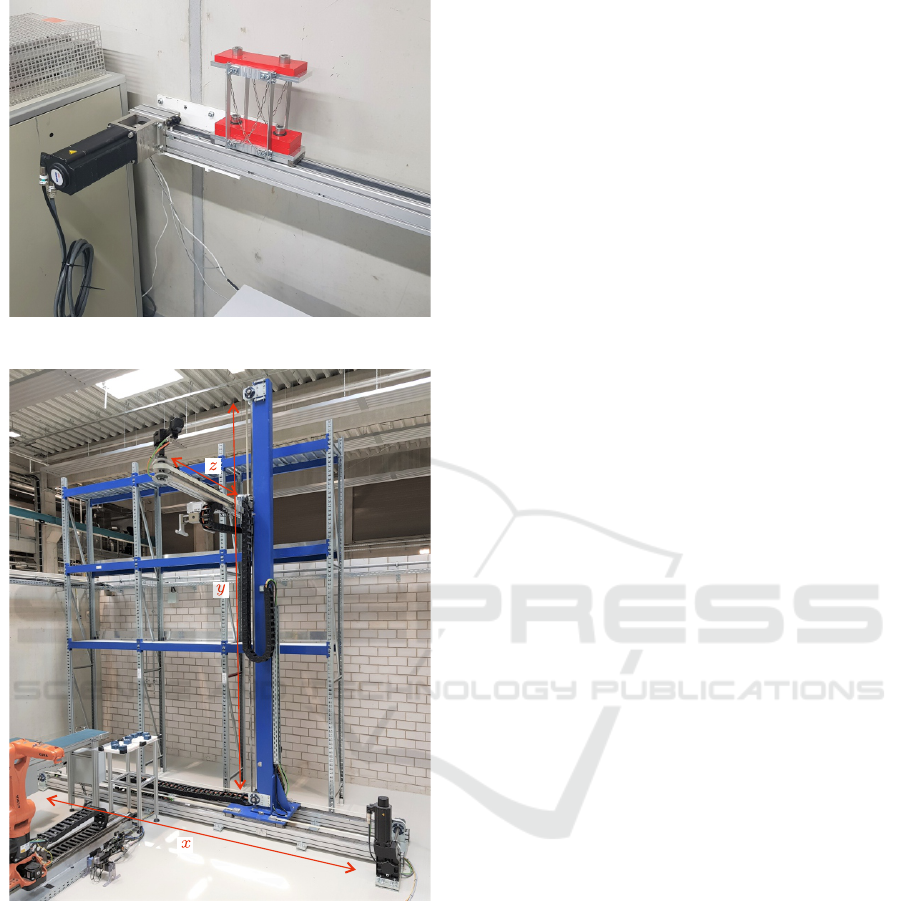
(a) Positioning stage with load on leaf springs

(b) Stacker crane

Figure 3: Experimental testbeds.

4.1 Testbeds

Validation experiments are carried out on the two

testbeds shown in Fig. 3. In the positioning stage a

synchronous motor is connected to a toothed belt in

direct drive moving a gantry with adjustable load. In

addition, an extra load is mounted on leaf springs.

The stacker crane has a mast height of 5.6 m and

the x-axis is 5 m long. All three axes are driven

by synchronous motors with gearboxes and toothed

belts. Experiments are carried out on the x-axis be-

cause due to mast oscillations and the elastic belt this

is the most challenging control design task. The y-

axis is positioned constantly at 2000 mm, 0 being the

bottom end.

In both setups the motors are equipped with re-

solvers on the motor axis for position and veloc-

ity measurement. All motors, sensors and drives

are of-the-shelf products from the company Lenze,

which brings about a cascaded control structure (cur-

rent, velocity, position). Position control is disabled,

while the speed controller’s TF is given by C(s) =

(1 + 1/(T

s)). Its output is a torque, which is cal-

culated into a current with the motor constant. Addi-

tional notch ﬁlters could be tuned for the commanded

current but this possibility is not utilized here. The

current controller is parametrized as recommended by

the manufacturer.

4.2 Reconstruction of the Step Response

from Frequency-domain

Measurements

Before the results of the model selection are shown,

the reconstruction of step responses for different con-

troller settings is veriﬁed along measurements on the

positioning stage testbed. The results for the stacker

crane look similar, but they are not shown for the sake

of brevity.

Following Sec. 3.3 and (8) the closed-loop FRF

from desired velocity r

to actual velocity has been

measured for K

= 0.0186 Nm, T

→ ∞ one time with

stepped sine, stepping from 0.5Hz to 500Hz. On

this basis step responses have been reconstructed as

described in Sec. 3.2 and Sec. 3.3 for different con-

troller settings with the square wave method and al-

ternating steps between −1 and 1. The base fre-

quency is 0.5 Hz, so steps in either direction occur at

1Hz. Fig. 4, 5, and 6 show the resulting calculated

step responses along with actually measured step re-

sponses for the respective controller settings. In or-

der to qualitatively demonstrate the effect of nonlin-

earities and disturbances, two different step heights

are shown each. For better comparison the calculated

step responses are scaled to the same speed range as

the measurements. Scaling is possible here because

the static gain is known to be 1.

It can be seen that the calculated step responses

resemble the measurements (overshooting, settling

time, frequency of vibration) quite well. A notewor-

thy difference is the remaining oscillation in the mea-

surement. This oscillation is synchronous with the

motor angle (four peaks per revolution) and is there-

fore not part of the settling motion but rather a cause

of a slight commutation misalignment of the current

ICINCO 2022 - 19th International Conference on Informatics in Control, Automation and Robotics

610

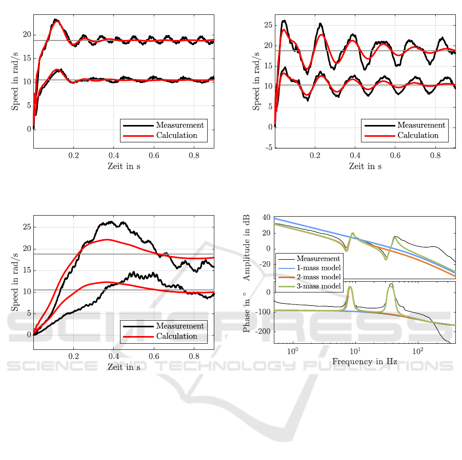
Figure 4: Measured and calculated step responses for two

different step heights, K

= 0.0186 Nm/rpm, T

→ ∞.

Figure 5: Measured and calculated step responses,

= 0.00186 Nm/rpm, T

→ ∞.

measurement. It shows the disturbance rejection /

ampliﬁcation property, not the settling motion. Dif-

ferences between the measurements for different step

heights caused by nonlinearity can clearly be seen, es-

pecially for t > 1 s in Fig. 6. Deviations of this size

should therefore also be expected between calculation

and measurement. In Fig. 5 the overshooting is not

captured precisely. This shows the lack of accuracy if

origin

and C

dest

differ signiﬁcantly in their controller

settings (here factor 10).

4.3 Model Selection for the Positioning

Stage Testbed

The identiﬁcation of multiple mass models is carried

out by inserting an excitation at r

, see Fig. 2, while

position control is disabled and the speed control is

kept at a low bandwidth (proportional gain set to a

factor 100 below the usual value). Because of the low

bandwidth it can be ensured that every frequency line

Figure 6: Measured and calculated step responses,

= 0.0186 Nm/rpm, T

= 14 ms.

Figure 7: Plant FRF and identiﬁed models for the position-

ing stage.

is excited sufﬁciently and the experiment is close to an

open-loop experiment, leading to a smooth FRF mea-

surement without signiﬁcant closed-loop bias. The

speed controller still prevents drifting of the integrat-

ing system.

A known PT1 element is included in all TF mod-

els with time constant T

to account for the known

sensor low-pass ﬁlter and current control, although a

PT2 model would be more accurate. The known time

constant is T

= 1.7ms, 1.2ms as sensor ﬁlter time

constant and 0.5ms for the current control.

Plant input and output (current and velocity) are

evaluated with the G

ortzel algorithm (Sysel and Ra-

jmic, 2012) over several periods to average out mea-

surement noise. The three different models shown

in Fig. 7 have been identiﬁed by minimizing the

mean squared distance in the complex plane over all

recorded frequencies via particle swarm optimization.

It can be seen that the 3-mass model ﬁts best but at

high frequencies a bias occurs in all models.

Based on these models the various controllers are

Control-relevant Model Selection for Multiple-mass Systems

611

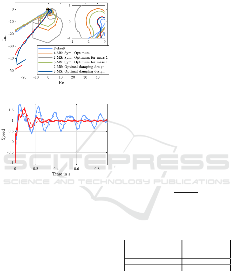
Figure 8: Nyquist plot for the considered set of model-based

controllers, positioning stage testbed.

Figure 9: Calculated step responses for those settings that

where approved in Fig. 8 (dashed) and corresponding mea-

surements (continuous). The colours correspond to Fig. 8.

calculated. The pole placement methods for 2-mass

systems described in Sec. 2.2 could not be applied

because the inertia ratio of the identiﬁed 2-MS is

≈ 0.5 < 1.0.

In Fig. 8 the open-loop FRFs are shown as a ﬁrst

validation step. In addition, the default controller set-

ting, provided by the manufacturer is shown for com-

parison. It is optimized for running the motor without

load.

It can be seen that the symmetric optimum vari-

ants have insufﬁcient gain margin. For this rea-

son only the remaining three settings are further in-

vestigated by calculating the step response from the

closed-loop FRF, measured with default controller

settings, see Fig. 9. The colours correspond to Fig. 8.

Actually measured step responses are shown for com-

parison, normalized to steps form −1 to 1. Because

the red and the dark blue curve could hardly be dis-

tinguished, only the red curve is plotted.

Comparing the measured and calculated step re-

sponses it can be said that the frequency of oscillation

and the decay ratio are in good agreement, whereas

the overshoot is underestimated. Nevertheless, the

evaluation of calculated step responses allows a ﬁrst

estimate. The exact shape of the step responses de-

pends also on the step height due to nonlinearities, as

shown in Sec. 4.2 and is therefore not captured pre-

cisely by the linear method.

Comparing the different control settings it can be

seen that the optimal damping design achieves a clear

improvement over the default setting and also the 1-

mass model would not be appropriate. However, there

is no clear answer to whether the 2-mass model or the

3-mass model should be favoured, because in this case

both optimal damping designs lead to similar control

parameters and therefore also similar performance.

4.4 Model Selection for the Stacker

Crane Testbed

Repeating the same workﬂow for the stacker crane

testbed Fig. 10 shows the open loop locus for a num-

ber of control settings, see legend in Fig. 11. Some

curves are not shown to keep the ﬁgure clean. The

latter ﬁgure shows the calculated step responses. Er-

ror norms for the four admissible controller settings

(sufﬁcient gain margin in Fig. 10) are given in Tab. 1.

The error norms for discrete-time signal y

are deﬁned

as follows:

∑

− 1|, (9)

∑

− 1)

, (10)

overshooting = max

− 1). (11)

Table 1: Performance criteria for the calculated step re-

sponses in m/s, stacker crane.

overs.

Default setting 114 5.7 0.344

3-MS: Sym. Optimum 76 3.88 0.199

2-MS: Optimal damping 111 6.73 0.299

3-MS: Optimal damping 142 8.22 0.238

Which controller and accordingly which model

should be selected depends on the requirements of the

application, but in this case it can be said that the sym-

metric optimum design based on the third mass of a

3-mass system is superior in all error norms. So, the

control-optimal model for this testbed is clearly the

3-mass model.

A comparison of measured and calculated step re-

sponses is shown in Fig. 12. The overall shape is in

ICINCO 2022 - 19th International Conference on Informatics in Control, Automation and Robotics

612

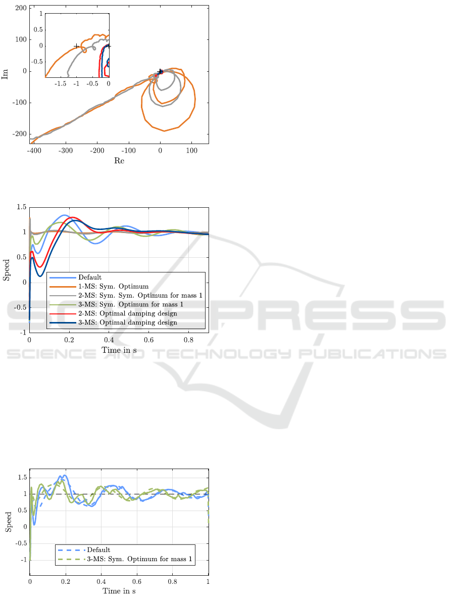
Figure 10: Nyquist plot for the considered set of model-

based controllers, stacker crane.

Figure 11: Calculated step responses for different model-

based controllers, stacker crane.

good agreement, except for additional scattering in

the measurement which is assumed to be caused by

backlash. So, although nonlinearity has a signiﬁcant

inﬂuence on the step response, the linear method does

not fail. Merely the nonlinear artefacts are not pre-

dicted correctly.

Figure 12: Calculated (continuous) vs. measured and scaled

(dashed) step responses for two controller settings, stacker

crane.

5 DISCUSSION

This paper is intended to give a possible answer to

the often asked question: Given a frequency-domain

measurement of a system and several candidate mod-

els obtained from parameter identiﬁcation, which

model is the one to choose for control design? The

proposed decision making comes at little expense as

only one more experiment is required rather than sev-

eral experiments (one for each controller-model com-

bination). The reason why this second experiment is

necessary at all is twofold: Firstly, a higher accuracy

of the veriﬁcation with calculated step responses can

be achieved by the special experiment in closed loop,

as explained in Sec. 3.3, which is also expectable from

the cited literature about identiﬁcation for control.

This theory says that a model should always be mea-

sured in a way that is close to its intended purpose.

Secondly, model selection requires a separation into

training and validation dataset. The second experi-

ment constitutes the validation dataset and is therefore

indispensable for a precise and unbiased performance

scoring. A third dataset (test data) comprises of the

measured step responses, which are not really part of

the model selection method but serve as a validation

of the method as a whole.

The results of the preceding section have demon-

strated a fairly good accuracy of the step response

calculation in spite of parasitic nonlinearities for two

testbeds. These nonlinearities result from the fact that

no ideal mass-spring-damper systems where tested

but realsitic, application-oriented setups with indus-

trial hardware. This is especially true for the stacker

crane.

Model selection was carried out successfully, al-

though the simple PI control cannot fully utilize the

relatively complex models. This is evident from the

fact that all the step responses look relatively simi-

lar. In both examples the exact model is not as critical

as one might expect from Fig. 7, where the models

have a clearly different ﬁt. The method cannot eas-

ily be extended to other controller transfer functions,

possibly with higher order. For example, PID con-

trol cannot readily be incorporated because the suit-

ability of the derivative feedback depends also on the

sensors’ signal quality, which cannot be taken into

account easily. This is unfortunate because some-

times PID control can be an advantage over PI con-

trol (Zhang and Furusho, 2000). It could be investi-

gated in future works if methods with more explicit

model-dependency like ﬂatness-based control of 2/3-

mass systems (Tkany et al., 2020) show a more sig-

niﬁcant difference between the models.

It should be highlighted that this model selection

Control-relevant Model Selection for Multiple-mass Systems

613

method is very close to existing approaches, where

several physically motivated models are identiﬁed

without any considerations about control-relevant ex-

citation or control-relevant cost functions and then a

commissioning engineer has to decide which model

is most suitable. However, better results could possi-

bly be obtained if the parameter identiﬁcation of the

candidate models was already carried out with spe-

cial control-relevant cost functions, see for example

(Codrons, 2005), not only the model selection. It can

be seen in Fig. 7 that the parameter identiﬁcation, as

carried out in this paper, leads to bias errors in am-

plitude at high frequencies, where the phase is around

−180

◦

in Fig. 8. As a consequence of the inaccuracy

some of the designed controllers are rendered inap-

propriate although they could possibly work well with

a more accurate model. It is possible that a more spe-

cialized identiﬁcation criterion could avoid this bias

and instead introduce bias at less important frequen-

cies. Considering control-relevant identiﬁcation cri-

teria could be future work.

Another problem is that the best controller for a

certain model may not have been tested, because only

a limited number of controllers is considered. Also,

the parametrization of hyperparameters is sometimes

arbitrary, for example the damping ratio. The possi-

bility exists that for a different damping ratio a better

performance could have been obtained. On the other

hand, a completely manual model selection procedure

would probably be suboptimal in the same way and

the given procedure is still more systematic.

6 CONCLUSION

In the paper at hand a procedure was proposed to

leverage state-of-the-art model-based controllers to

realize a control-oriented model selection of ﬁrst prin-

ciple models for electric drives with imperfect me-

chanics. The goal is to select the model that leads to

optimal performance of a model-based controller, not

the most accurate model. A clear focus was laid on

model selection rather than parameter identiﬁcation.

The model selection is based on open-loop frequency

response functions and step responses for veriﬁcation

of the different model-controller combinations.

In experiments on two industrial testbeds it was

shown that the step responses calculated with the

nonparametric model predict the general shape accu-

rately, while deviations still exist due to nonlinearities

and disturbances in the real system that are arguably

not related to the settling motion. A clear improve-

ment of the controller’s performance over the default

settings was achieved for one of the two testbeds.

Limitations are the inability to consider sensor noise

explicitly and the not control-optimal bias error in

the parameter identiﬁcation. The experiments have

shown that the best model is not always the most ac-

curate model, as expected. But it was found that often

there is no sharp optimum and several models are al-

most equally good.

ACKNOWLEDGEMENTS

This work was sponsored by the German Forschungs-

vereinigung Antriebstechnik e.V. (FVA).

REFERENCES

Abate, J. and Whitt, W. (2006). A uniﬁed framework for

numerically inverting laplace transforms. INFORMS

Journal on Computing, 18(4):408–421.

Aguilar, J., Cerrada, M., and Cordero, A. T. F. (2001). Ge-

netic programming-based approach for system identi-

ﬁcation. Advances in Fuzzy Systems and Evolutionary

Computation, Artiﬁcial Intelligence, pages 329–334.

Brun, R., Reichert, P., and K

unsch, H. R. (2001). Practical

identiﬁability analysis of large environmental simula-

tion models. Water Resources Research, 37(4):1015–

1030.

Chatﬁeld, C. (1995). Model uncertainty, data mining and

statistical inference. Journal of the Royal Statistical

Society: Series A, 158(3):419–444.

Codrons, B. (2005). Process modelling for control: a uni-

ﬁed framework using standard black-box techniques.

Springer Science & Business Media.

Date, P. and Vinnicombe, G. (2004). Algorithms for worst

case identiﬁcation in H

∞

and in the ν-gap metric. Au-

tomatica, 40(6):995–1002.

Doetsch, G. (1985). Anleitung zum praktischen Ge-

brauch der Laplace-Transformation und der Z-

Transformation. R. Oldenbourg Verlag M

unchen,

ﬁfth edition.

Geng, L.-H., Cui, S.-G., Zhao, L., and Lin, H.-Q. (2015). A

convex optimization algorithm for frequency-domain

identiﬁcation in the v-gap metric. International

Journal of Adaptive Control and Signal Processing,

29:362–371.

Gevers, M. (2004). Identiﬁcation for control: Achievements

and open problems. IFAC Proceedings, 37(9):401–

412.

Gevers, M. and Ljung, L. (1986). Optimal experiment de-

signs with respect to the intended model application.

Automatica, 22(5):543–554.

omez, P., Arellano, P., and Mota, R. O. (2007). Fre-

quency domain transient analysis applied to transmis-

sion system restoration studies. In Proc. of the 7th In-

ternacional Conference of Power Systems Transients

(IPST’07).

ICINCO 2022 - 19th International Conference on Informatics in Control, Automation and Robotics

614

Grassmann, W. K. (2013). Computational probability, vol-

ume 24. Springer Science & Business Media.

Hjalmarsson, H., Gevers, M., and De Bruyne, F. (1996).

For model-based control design, closed-loop iden-

tiﬁcation gives better performance. Automatica,

32(12):1659–1673.

Hosono, T. (1981). Numerical inversion of laplace trans-

form and some applications to wave optics. Radio

Science, 16(6):1015–1019.

Jansson, H. (2004). Experiment design with applications in

identiﬁcation for control. PhD thesis, Royal Institute

of Technology (KTH), Stockholm, Sweden.

Khan, M. B., Munawar, K., and Nisar, H. (2013). Switched

hybrid position control of elastic systems with back-

lash. In 2013 IEEE International Conference on Con-

trol System, Computing and Engineering, pages 551–

556. IEEE.

Manabe, S. a. (1998). Coefﬁcient diagram method. IFAC

Proceedings Volumes, 31(21):211–222.

Oomen, T., van Herpen, R., Quist, S., van de Wal,

M., Bosgra, O., and Steinbuch, M. (2013). Con-

necting system identiﬁcation and robust control for

next-generation motion control of a wafer stage.

IEEE Transactions on Control Systems Technology,

22(1):102–118.

Risuleo, R. S. (2016). System identiﬁcation with input un-

certainties: an EM kernel-based approach. PhD the-

sis, KTH Royal Institute of Technology.

Riva, M. H., Dagen, M., and Ortmaier, T. (2016). Adap-

tive unscented kalman ﬁlter for online state, parame-

ter, and process covariance estimation. In American

Control Conference (ACC), pages 4513–4519. IEEE.

Saha, P., Egerstedt, M., and Mukhopadhyay, S. (2021).

Neural identiﬁcation for control. IEEE Robotics and

Automation Letters, 6(3):4648–4655.

Schr

oder, D. (2015). Elektrische Antriebe-Regelung von

Antriebssystemen. Springer Vieweg, Berlin, Germany,

fourth edition.

Sch

utte, F. (2003). Automatisierte Reglerinbetriebnahme

ur elektrische Antriebe mit schwingungsf

ahiger

Mechanik. Shaker.

Sch

utte, F., Beineke, S., Grotstollen, H., Fr

ohleke, N.,

Witkowski, U., R

uckert, U., and R

uping, S. (1997).

Structure-and parameter identiﬁcation for a two-mass-

system with backlash and friction using a self-

organizing map. In European Conference on Power

Electronics and Applications, volume 3, pages 3–358.

Sysel, P. and Rajmic, P. (2012). Goertzel algorithm gen-

eralized to non-integer multiples of fundamental fre-

quency. Journal on Advances in Signal Processing

(EURASIP), 2012(1):1–8.

Tacx, P., de Rozario, R., and Oomen, T. (2021). Model order

selection in robust-control-relevant system identiﬁca-

tion. In 19th IFAC Symposium on System Identiﬁca-

tion, volume 54, pages 1–6. Elsevier.

Tan, N., Atherton, D. P., and Y

uce, A. (2017). Computing

step and impulse responses of closed loop fractional

order time delay control systems using frequency re-

sponse data. International Journal of Dynamics and

Control, 5(1):30–39.

Tantau, M., Jonsky, T., Ziaukas, Z., and Jacob, H.-G.

(2022). Control-relevant model selection for servo

control systems. In International Conference on Con-

trol, Decision and Information Technologies, pages 1–

8, Istanbul, Turkey. IEEE. accepted.

Tantau, M., Popp, E., Perner, L., Wielitzka, M., and Ort-

maier, T. (2020). Model selection ensuring practi-

cal identiﬁability for models of electric drives with

coupled mechanics. In 21st International Federation

of Automatic Control (IFAC) World Congress, Berlin,

Germany.

Tkany, C., Grotjahn, M., and K

uhn, J. (2020). Flatness-

based feedforward control of a stacker crane with

online trajectory generation. In 2020 4th Interna-

tional Conference on Automation, Control and Robots

(ICACR), pages 79–87. IEEE.

Toscano, R. and Lyonnet, P. (2009). Robust pid controller

tuning based on the heuristic kalman algorithm. Auto-

matica, 45(9):2099–2106.

Tripathi, S. M., Tiwari, A. N., and Singh, D. (2015). Op-

timum design of proportional-integral controllers in

grid-integrated pmsg-based wind energy conversion

system. International Transactions on Electrical En-

ergy Systems, 26(5):1006–1031.

Van den Hof, P. (1997). Closed-loop issues in system iden-

tiﬁcation. IFAC Proceedings, 30(11):1547–1560.

Van Den Hof, P. M. J. and Schrama, R. J. P. (1994). Identiﬁ-

cation and control-closed loop issues. IFAC Proceed-

ings, 27(8):311–323.

van Herpen, R., Oomen, T., and Bosgra, O. (2011). A

robust-control-relevant perspective on model order se-

lection. In Proceedings of the American Control Con-

ference, pages 1224–1229. IEEE.

van Herpen, R., Oomen, T., van de Wal, M., and Bosgra,

O. (2010). Experimental evaluation of robust-control-

relevance: A confrontation with a next-generation

wafer stage. In Proceedings of the American Control

Conference, pages 3493–3499. IEEE.

Vinnicombe, G. (2001). On closed-loop identiﬁcation: er-

ror distributions in the ν-gap metric. In 40th IEEE

Conference on Decision and Control, volume 4, pages

3099–3103. IEEE.

Wertz, H. and Schutte, F. (2000). Self-tuning speed con-

trol for servo drives with imperfect mechanical load.

In IEEE Industry Applications Conference, volume 3,

pages 1497–1504. IEEE.

Witczak, M., Obuchowicz, A., and Korbicz, J. (2002). Ge-

netic programming based approaches to identiﬁcation

and fault diagnosis of non-linear dynamic systems. In-

ternational Journal of Control, 75(13):1012–1031.

Yang, Z., Geng, L., and Yang, Y. (2018). A computation-

ally efﬁcient eiv models identiﬁcation method using

the v-gap metric. In 37th Chinese Control Conference

(CCC), pages 1729–1734. IEEE.

Zhang, G. and Furusho, J. (2000). Speed control of two-

inertia system by pi/pid control. IEEE Transactions

on industrial electronics, 47(3):603–609.

Control-relevant Model Selection for Multiple-mass Systems

615

REFERENCES

Abate, J. and Whitt, W. (2006). A unified framework for