Sales Prediction Model based on Multifactorial Linear Regression

Jiyan Liu

Department of Mathematics and Department of Economics, University of California San Diego, La Jolla, U.S.A.

Keywords: Sales Prediction, Linear Regression, Multifactorial Regression.

Abstract: Motivated by the sales prediction of ABCtronics, this paper aims to provide integrated process for creating a

proper multiple linear regression model and detailed analysis of according parameters. With multiple

independent variables, the linear regression model exams the relationship between a collection of data-overall

market demand, price per chip and economic condition to the single dependent variable sales volume of

ABCtronics. The target is set to be future prediction of sales volume with three observable variables. All

outputs are statistical results from Minitab which contain regression equation, model summary with R

value

and analysis of variance stating the significance level of each variable. With detailed output, a refined multiple

regression model is then developed to get rid of the overall market demand term. Pure regression equation

brings only numerical understanding, i.e., visualization is the next focus. Based on comparison and contrast,

it is verified the accurateness of the refined model. These results shed light on the proper use of multiple linear

regression on sale prediction model.

1 INTRODUCTION

Sales prediction plays a key role in almost every

successful operation of business. As one of the

greatest inventions, it provides forecasting on future

trend of target markets and an insight into proper

allocation of resources e.g., labors and capitals. The

way to maximize firm’ sale target with limited

resources is always considered the priority.

Forecasting sales accurately for a new product is

difficult and complex due to non-availability of past

data. However, such forecast information is crucial for

successful introduction of new products which, in

turn, determines the survival of companies, in many

cases (Meeran, et al, 2013). Hence, proper usage of

sales prediction model can assist the firms with

informed data on each input which may help refine

future supply chain. Moreover, as the number of

databases collected increases, corporations are able to

gain less biased data which not only gives sales

prediction but consumer preferences. Specifically, if

linear regression model is formed, parameter of each

variable would be given and that number tells the unit

change of the regressors. By comparing the

parameters, firms may attribute any boost of sales

volume to some specific determinant factor, which can

https://orcid.org/0000-0001-7666-3749

be use to select suitable market target group and

increase efficiency further.

Sales prediction models are now widely used in all

fields. From prior literature, there are already intensive

research on sales prediction in three major fields. First

is the Microsoft Time Series algorithm. It provides us

with optimized regression algorithm for forecasting

continuous real-time values (Kohli, Shreya, et al,

2020). Time Series forecasting, which forecasts based

on time-controlled variable, is an important tool under

this scenario, where the research aim is to predict the

behavior of complex systems solely by analyzing the

past data (A Survey of Time Series Data Prediction on

Shopping Mall, et al, 2013). For example, three

researchers from Indian conduct a survey of time

series data prediction on shopping mall to predict the

next phase of the product price trends and sales

volume. They propose a tree based data mining

algorithm that treats market’s behavior and interest as

input & filter the desired output efficiently & a mining

model of stream data time-series pattern in a dynamic

shopping mall (A Survey of Time Series Data

Prediction on Shopping Mall, et al, 2013). This is a

comparatively complicated model because what

involves are subjective investors who may cause

significant error on the analyzing system, which leads

to its complexity.

598

Liu, J.

Sales Prediction Model based on Multifactorial Linear Regression.

DOI: 10.5220/0011195100003440

In Proceedings of the International Conference on Big Data Economy and Digital Management (BDEDM 2022), pages 598-604

ISBN: 978-989-758-593-7

Second is spatial data mining for retail sales

forecasting. The study conducted by Maike Krause-

Traudes, Simon Scheider1 and two other scientists

aim to design a regression model to predict probable

turnovers for potential outlet-sites of a big European

food retailing company (Aina, Abidemi Ayodeji, et al,

2012). The forecast of potential sites is based on sales

data on shop level for existing stores and a broad

variety of spatially aggregated geographical, socio-

demographical and economical features describing the

trading area and competitor characteristics (Aina,

Abidemi Ayodeji, et al, 2012). As a result, Support

Vector Regression (SVR) is applied to provide the

prediction of sales of existing outlets with attributes

(e.g., floor space, number of parking lots, distance to

the next competitor etc.) as well as the relationship

between sales volume and these attributes. Finally, a

novel trigger model for sales prediction with data

mining techniques that focuses on how to forecast

sales with more accuracy and precision is proposed

(Kohli, Shreya, et al, 2020). Then, researchers lay

emphasis on online sales prediction instead of actual

daily sales volume.

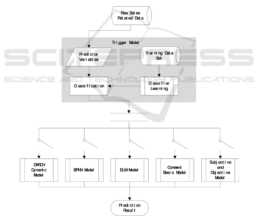
The approximate model they used is shown in Fig.

1. Raw data is first manipulated into available forms,

and then a trigger model is proposed to do the

classification. Next, the classification result shows the

potentially best prediction model for each SKU.

Finally, by use of the most appropriate model, the

prediction is accomplished.

With the model, data is classified and grouped to

facilitate analysis. The trigger model is a combination

of several basic models with Mean Absolute

Percentage Error (MAPE) to evaluate the performance

of proposed method. Compared with the baseline

model ARMA, the trigger model possesses more

accuracy (Huang 2015).

Figure 1: A sketch of the framework of Trigger Model System (Huang 2015).

Sales Prediction Model based on Multifactorial Linear Regression

599

The model considered to use to predict sales

volume in this passage is multiple linear regression

models. Regression analysis is a statistical technique

for estimating the relationship among variables which

have reason and result relation (Uyanık, Gülden Kaya,

Neşe Güler, 2013). As a linear model, multiple

regression provides most direct insight on how change

in single unit of any independent variables affect the

sales volume. Recent research shows extensive use of

multiple linear regression in different fields. For

example, the relationships between Chlorophyll-a and

16 chemical, physical and biological water quality

variables in Camilleri reservoir (Ankara, Turkey)

were studied by using principal component scores

(PCS) in multiple linear regression analysis (MLR) to

predict Chlorophyll-a levels (Çamdevýren, Handan, et

al, 2005). In addition, the simulation of water table

responses is discussed and the use of multiple linear

regression as a modelling technique is considered. The

model permits the consideration of changes in

properties of recharge, discharge and aquifer

parameters simultaneously (Hodgson, Frank D, 1978).

The rest part of the paper is organized as follows:

In the first following part, case used for multiple

regression model in this passage will be introduced

with data and model presented. For visualization,

output from Minitab and graphs would be presented,

along with assumptions for proper utilization of the

model, and how the model is evaluated. Moreover,

results output of software, not only the output

function, given R

value and VIF but also the Four in

one graph for the observational data versus the

predicted data with residuals would be explained and

presented one by one with clarification. One can

understand what the data represents and what the

graph indicates without any background knowledge.

Based on analysis provided and output given by graph,

final conclusion would be given with discussions on

limitation of the model. Finally, conclude upon all the

paragraph including future expectations on prediction

of the sales model.

2 DATA AND METHOD

The whole analysis of sales volume and model

prediction is based on the ABCtronics case. In this

case, reader serves as an intern of the ABCtronics firm

which specializes in producing IC chips. Recent

consumer feedback and data shows a dramatic

increase in the rejection rate from XYZfirm, which

causes doubt from the Audit committee (Adhikari,

Arnab, et al, 2016). As the main focus of this passage

the use of multiple linear regression model, analysis

on consumer feedback and rejection rate are ignored,

the main focus would be prediction of future sales

volume by multiple linear regression. Table I provided

historical sales.

Table 1: Historical Sales Figure of Abctronics (Adhikari,

Arnab, Et Al 2016).

ABCtronics’ sales

Year volume (in

millions)

Overall market

demand

(in millions)

Price per

chip (in

Economic

condition

2004 2.39 297 0.832 0

2005 3.82 332 0.844 1

2006 3.33 195 0.854 0

2007 2.49 182 1.155 1

2008 1.56 93 1.303 0

2009 0.97 98 1.265 0

2010 1.32 198 1.368 1

2011 1.42 188 1.208 0

2012 1.48 285 1.234 1

2013 1.85 264 1.282 1

Note.∗Economic condition : 1 signﬁes favorable market condition and 0 signﬁes

otherwise.

For multiple linear regression model to be

applicable, at least two independent variables are

needed. For multiple linear regression, the proposed

model is shown below:

𝑌=𝛽



+𝛽



𝑋



+𝛽



𝑋



+𝛽



𝑋



+𝜀





where ε~ Normal (0, σ²). Here, an error term of

normal distribution with mean 0 and standard

deviation σ² is included accounting for instability of

this model.

From the table, statistics show three different

independent variables and one dependent variable-

ABCtronics’ sales volume. Since statistically

significance of any independent variable cannot be

determined only by looking at the raw data. The first

try includes all three independent variables in the

model and the corresponding results are shown in Eq.

(1) Table Ⅱ Table Ⅲ and Table Ⅳ.

Table 2: Coefficients for all independent variables inclusing

the constant term.

Term Coef SE Coef T-Value P-Value VIF

Constan

8.86 1.35 6.57 0.001

Overall

market

demand

-0.00524 0.00258 -2.03 0.089 3.27

Price Per

Chip

-5.505 0.881 -6.25 0.001 2.54

Economic

Condition

1.130 0.342 3.30 0.016 2.44

BDEDM 2022 - The International Conference on Big Data Economy and Digital Management

600

Table 3: Overall Model summary for three independent

variables.

S R-sq R-sq(adj) R-sq(pred)

0.346274 90.75% 86.13% 72.75%

Table 4: Additional Information Including The F-Value.

Source

Adj SS Adj MS

F-

Value

P-

Value

Regression 3 7.0606 2.3535 19.63 0.002

Overall market

demand

1 0.4930 0.4930 4.11 0.089

Price Per Chip 1 4.6786 4.6786 39.02 0.001

Economic

Condition

1 1.3089 1.3089 10.92 0.016

Erro

6 0.7194 0.1199

Total 9 7.7800

sale = 8.86 − 0.00524 market demand

−5.505 Price Per Chip

+ 1.130 Economic Condition





Adjusted R

from model summary shows that only

86.13% of the variation in the sales volume is

explained by this regression model. Adjusted R

preferred here since it takes into account the real

variation by adding more variables, which h still

shows high percentage of prediction coverage. To

justify the accurateness of this model, p-values for

each different variable are required, which is shown as

the last column of Analysis of Variance part. Taking a

95% confidence level, p-value of Overall market term

equals 0.089 which is greater than 5%, the passing line

for statistically significance. For any p-value greater

than 5%, independent variable with that specific p-

value is considered statistically insignificant. Getting

rid of that term would provide more accurate result

since insignificant variable attributes little to predict

future sales volume. A refined model is provided

taking only Price per chip and economic condition as

independent variables. With the same regression

model, data output from Minitab is shown in Table Ⅴ,

Table Ⅵ and Eq. (2).

sales = 6.452 − 4.136 Price Per Chip

+0.606 Economic Condition





Table 5: Overall Model summary or two variables.

S R-sq R-sq(adj) R-sq(pred)

0.416172 84.42% 79.96% 64.42%

Table 6: Coefficients summary for two variables and the

constant term.

Term Coef

Coef

T-

Value

P-

Value

VIF

Constan

6.452 0.766 8.42 0.000

Price Per

Chip

-4.136 0.680 -6.08 0.001 1.05

Economic

Condition

0.606 0.269 2.25 0.059 1.05

The p-value here are comparatively small, which

proves the two independent variables to be statistically

significant. Furthermore, for it not be a biased model,

multicollinearity still needs to be tested.

Multicollinearity defines the correlation between two

independent variables so if too high, the prediction

will not be accurate as variation in one variable affects

the other as well. Variance inflation factor (VIF)is

then chosen to exam the correlation. Here, coefficient

component of above graph gives result of VIF to be

1.05, which is much smaller than the standard value 5.

To sum up, there is no multicollinearity between these

two variables and the refined model seems to be

suitable for predicting the sales figure of ABCtronics.

Table 7: Coefficient for single variable ‘overall market’

term.

Term Coef SE Coef T-Value

P-

Value

VIF

Constan

0.753 0.779 0.97 0.362

Overall

market

demand

0.00614 0.00344 1.79 0.112 1.00

3 RESULTS AND DISCUSSION

For the modified model:

Sales Volume = 6.452 − 4.136 price per chip2

+0 .6063 economic condition





Adjusted R

in this model shows that around

79.96% of the variation in the sales volume is

explained by this regression model, which is

comparatively high for a sales prediction model.

Further clarification for choosing confidence level at

95% is needed. According to the analysis, a simple

linear regression model with overall market demand

was ran before any multiple linear regression.

Sales Prediction Model based on Multifactorial Linear Regression

601

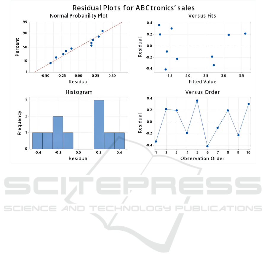
Figure 2: Residual plots for ABCtronics’ sale for all three independent variables.

P-value of this single independent variable is

0.112, which is higher than 10%, corresponding value

of 90% confidence level. Here, eve with a 10% level

of significance, overall market demand is still defined

as statistically insignificant, not to mention the 5%

level. It might work for lower levels of significance

but overall precision would decrease choosing too

low a significant level for any model. Therefore,

getting rid of the demand term may help people to

better estimate sales volume using a multiple

regression model.

From the model, unit increases in price per chip

would lead to approximately 4.136 units decrease in

the sales volume. For the binary economic condition

value, signifies favorable market condition would

lead to 0.6 unit increase in sales volume. For instance,

ABCtronics should operate in favor of market

condition and control their chip price comparatively

low to maximizes sales volume.

To visualize and better compare two different

regression modes with and without overall market

demand variable, Four-in -one graphs with normal

probability plot, histogram, versus fit and versus

order are shown in Fig. 2. With all three independent

variables, top left plot shows how fit the real data to

the fitted line; top right is the verification that

residuals are randomly distributed; bottom left is the

histogram with frequency and bottom right is data of

residual in order.

The top left normal probability curve is a

visualization of R

value: predicted value forms the

best fitted line shown as the red straight line. For each

point, it represents the real sales volume from 2004 to

2013.The more variation that is explained by the

model, the closer the data point fall to the fitted

regression line. The distance between reel value point

and the predict line is defined as residuals. The lower

the residuals, better fit is the model of prediction.

From above top left plot, real points are all shown to

be close to the predicted line, which signals high R

corresponding to our result-90,75%.

The top right residual fits graph plots residual on

y axis and fitted value on x-axis. The residuals versus

fits plot is used to verify the assumption that the

residuals are randomly distributed and have constant

variance. Therefore, ideally, the points should fall

randomly on both sides of 0. To sum up, the versus fit

plot is at ideal status.

The bottom left histogram graph is easy to

understand -it shows the frequency of each residual.

Larger frequency with small residuals is favorable

since it represents more accurate prediction. But here,

data with 0 residual does not exist due to flaws on

design of the model.

BDEDM 2022 - The International Conference on Big Data Economy and Digital Management

602

The versus order graph is similar to the versus fits

graph but plotted in order that of the date collected.

Independent residuals show no trends or patterns

when displayed in time order. From the graph,

residuals near year 2005 and 2006 may be correlated

since the difference is comparatively low, but the

overall trend of residuals fall randomly around the

center line.

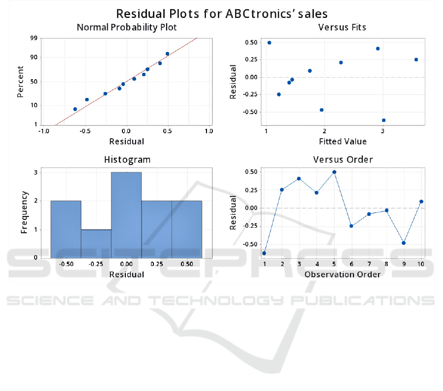
Figure 3: Residual plots for ABCtronics’ sales for two variables.

Getting rid of the overall market term,with two

independent variables ,the top left plot shows better

fit of the real data to the fitted line ;top right is still

the verification that residuals are randomly

distributed; bottom left is the histogram with residual

frequency more in the middle and bottom right is data

of residual in order.

Now, one is able to reproduce the four-in-one

graph with only two independent variables. The

residual plot seems to be closer to the fitted line which

shows increase in R

value. Versus fit and order graph

still show random distribution of the residual points

around the center line. The histogram is with more

differences-frequency of predicted data with small

residuals increase a lot comparatively, which shows a

pattern closer approximates to the normal

distribution. Hence, visualization for model of

prediction shows the same result as pure linear

equation that getting rid of the overall market variable

helps refine the multiple regression model.

Multiple linear regression model seems to provide

a proper prediction for future sales volume. However,

nothing can be guaranteed that table provided to

people from ABCtronics is flawless and contains all

factors influential to sales figures. First of all, whether

there is omitted variable that are not mentioned in the

model is unclear. If there is omitted variables which

also determines changes in the sales volume, the

model is then incomplete and biased since not all

factors are included. Moreover, without telling

whether each independent variable correlates with

existing error terms, people are not sure that this is a

good model for prediction. If correlation exists, IV

regression needs to be done to find other better

independent variables. Additionally, real world

economy is more complicated with nonlinear

relationship, only using multiple linear relationship

may not provide desirable results. There are many

clinical problems which do not allow the option of

corroboration by more invasive and disruptive

approaches. For such problems, a more penetrating

approach to data analysis may be the only way to do

justice to the data set (BLACK, A.M.S., P. FOÉx,

1982).

Sales Prediction Model based on Multifactorial Linear Regression

603

4 CONCLUSION

In summary, sales prediction models based on

multiple linear regression is investigated based on

multiple independent variables related to sales

volume. The article starts with examples from

historical successful sale model prediction to the use

of multiple linear regression models among different

fields. Next comes the description of ABCtronics case

which would be used for building own sales prediction

model. Though as a linear regression, multiple

regression models vary a lot depends on how many

independent variables to include. Keep adding

meaningless variables affects nothing about the model

but create more bias. As a result, final model created

in the passage excludes one independent variable from

data provided to promote accuracy. Though the best

fitted model is found using multiple linear regression

here, in real world, linear model is comparatively

incapable of producing accurate sale figure prediction.

Furthermore, if people keeping conducting more

investigations, researchers may find other correlated

independent variables which become determinant

factors to predict sales volume. Including those factors

can further refine the multiple regression model and

give accurate prediction. These results offer a

guideline for more complicated models developed in

sale volume prediction model and give a chance for

people to create their own prediction model even if

one does not specialize in it.

REFERENCES

Mohammed Ali, S.Narasimha Rao, Abdul Rahim “A

Survey of Time Series Data Prediction on Shopping

Mall.” ISSN: 0976-5166 Vol. 4 No.2 Apr-May 2013

http://www.ijcse.com/docs/INDJCSE13-04-02-

100.pdf.

Adhikari, Arnab, et al. “Case—Abctronics: Manufacturing,

Quality Control, and Client Interfaces.” INFORMS

Transactions on Education, vol. 17, no. 1, 2016, pp. 26–

33., https://doi.org/10.1287/ited.2016.0158cs.

Aina, Abidemi Ayodeji, et al. “Spatial Data Mining for

Retail Sales Forecasting.” SSRN Electronic Journal,

2012, https://doi.org/10.2139/ssrn.2060272.

BLACK, A.M.S., and P. FOÉx. “Some Capabilities and

Limitations of Multiple Regression Analysis:

Application to Canine Coronary Blood Flow.” British

Journal of Anaesthesia, vol. 54, no. 12, 1982, pp. 1319–

1329., https://doi.org/10.1093/bja/54.12.1319.

Çamdevýren, Handan, et al. “Use of Principal Component

Scores in Multiple Linear Regression Models for

Prediction of Chlorophyll-a in Reservoirs.” Ecological

Modelling, vol. 181, no. 4, 2005, pp. 581–589.,

https://doi.org/10.1016/j.ecolmodel.2004.06.043.

G. Kohli, Shreya, et al. “Sales Prediction Using Linear and

KNN Regression.” Algorithms for Intelligent Systems,

2020, pp. 321–329., https://doi.org/10.1007/978-981-

15-5243-4_29.

Hodgson, Frank D. “The Use of Multiple Linear Regression

in Simulating Ground-Water Level Responses.”

Ground Water, vol. 16, no. 4, 1978, pp. 249–253.,

https://doi.org/10.1111/j.1745-6584.1978.tb03232.x.

Huang, Wenjie, et al. “A Novel Trigger Model for Sales

Prediction with Data Mining Techniques.” Data

Science Journal, vol. 14, 2015, p. 15.,

https://doi.org/10.5334/dsj-2015-015.

Meeran, S., et al. “Sales Forecasting Using Combination of

Diffusion Model and Forecast Market – an Adaption of

Prediction/Preference Markets.” IFAC Proceedings

Volumes, vol. 46, no. 9, 2013, pp. 87–92.,

https://doi.org/10.3182/20130619-3-ru-3018.00619.

Uyanık, Gülden Kaya, and Neşe Güler. A Study on

Multiple Linear Regression Analysis, vol. 106, 10 Dec.

2013, pp. 234–240.,

https://doi.org/https://doi.org/10.1016/j.sbspro.2013.12

.027.

BDEDM 2022 - The International Conference on Big Data Economy and Digital Management

604