An Ensemble Classiﬁer based Method for Effective Fault Localization

Arpita Dutta

1 a

and Rajib Mall

2 b

School of Computing, National University of Singapore, Computing Dr, Singapore

Dept. of Computer Science and Engineering, Indian Institute of Technology, Kharagpur, India

Keywords:

Software Fault Localization, Debugging, Ensemble Classiﬁer, Program Analysis.

Abstract:

Fault localization (FL) is one of the most difﬁcult and tedious task during software debugging. It has been

reported in literature that different FL techniques show superior results under different circumstances. No

reported technique always outperforms all existing FL techniques for each type of bug. On the other hand,

it has been reported that ensemble classiﬁers combine different learning methods to obtain better predictive

performance that may not be obtained from any of the constituent learning algorithms alone. This has mo-

tivated us to use an ensemble classiﬁer for effective fault localization. We focus on three different families

of fault localization techniques, viz., spectrum based (SBFL), mutation based (MBFL), and neural-network

based (NNBFL) to achieve this. In total, we have considered eleven representative methods from these three

families of FL techniques. Our underlying model is simple and intuitive as it is based only on the statement

coverage data and test execution results. Our proposed ensemble classiﬁer based FL (EBFL) method classiﬁes

the statements into two different classes viz., Suspicious and Non-Suspicious set of statements. This helps

to reduce the search space signiﬁcantly. Our experimental results show that our proposed EBFL technique

requires, on an average, 58% of less code examination as compare to the other contemporary FL techniques,

viz., Tarantula, DStar, CNN, DNN etc.

1 INTRODUCTION

With the increasing complexity and size of software

systems, bugs are inevitable (Wong et al., 2016). In

the complete process of debugging, fault localization

(FL) is the most time-consuming and tiresome. Any

improvement in this task lead to a huge reduction in

total software development cost. Hence, several FL

methods were reported in last two-to-three decades

(Choi et al., 2010; Wong et al., 2016; Dutta et al.,

2019a; Dutta et al., 2021; Dutta et al., 2019b).

Weiser (Weiser, 1984) introduced the concept of

program slicing. Later, Lyle et al.(Lyle, 1987) and

others (Krinke, 2004; Sridharan et al., 2007) extended

the Weiser’s static slicing with program execution in-

formation and proposed dynamic slicing, thin slic-

ing, hybrid slicing etc. However, these techniques

most often returns a considerably large size of pro-

gram slice without any ranking. To solve these is-

sues, different spectrum based and machine learn-

ing techniques are used for FL. SBFL techniques

take program spectra info and test execution results

https://orcid.org/0000-0001-7887-3264

https://orcid.org/0000-0002-2070-1854

as input and generate ranked list of statements. Fa-

mous SBFL techniques are Ochiai, Jaccard, Taran-

tula, DStar (Wong et al., 2013; Jones et al., 2002)etc.

Using the same input information as SBFL tech-

niques, different neural network models are also

trained to identify the faulty locations. Most com-

monly used NN models are BPNN(Wong and Qi,

2009), DNN(Zhang et al., 2017), CNN(Zhang et al.,

2019) etc. Mutation testing(Wong et al., 2016) is also

used for FL. MUSE(Moon et al., 2014) and Metal-

laxis(Papadakis and Le Traon, 2015) are two most

popular MBFL techniques.

Even though a large number of FL techniques

have been reported but none of these outperforms all

FL techniques in all circumstances. For example,

some of the techniques work very well for logical and

relational operator related faults whereas some other

technique work for arithmetic-operator related bugs.

It has been reported that ensemble classiﬁer combines

different learning methods to obtain better predictive

performance that may not be obtained from any of the

constituent learning algorithms alone. This motivated

us to use an ensemble classiﬁer for effective FL. Be-

sides, the existing techniques are not effective enough

Dutta, A. and Mall, R.

An Ensemble Classiﬁer based Method for Effective Fault Localization.

DOI: 10.5220/0011166800003266

In Proceedings of the 17th International Conference on Software Technologies (ICSOFT 2022), pages 159-166

ISBN: 978-989-758-588-3; ISSN: 2184-2833

159

for large size programs.

In order to address these stated problems, we pro-

pose an ensemble classiﬁer based FL method. We

focus on three different families of fault localiza-

tion techniques, viz., SBFL, MBFL, and NNBFL to

achieve this. In total, we have considered eleven

representative techniques from these three families.

We further discuss the extension of our proposed ap-

proach to localize multiple-fault programs.

Rest of the chapter is organized as follows: Pro-

posed method is discussed in Section 2. In Sec-

tion 3, empirical evaluation and obtained results are

discussed. We present the comparison with related

works in Section 4. We ﬁnally conclude in Section 5.

2 PROPOSED APPROACH: EBFL

Ensemble classiﬁer is a well accepted machine learn-

ing model which has better predictive performance

than each of the base classiﬁer (Mitchell et al., 1997).

To take advantage of this, we proposed an Ensemble

classiﬁer Based Fault Localization (EBFL) method.

In our proposed EBFL method, we use three differ-

ent fault localization families viz., SBFL, MBFL, and

NNBFL. Our proposed model ﬁrst classiﬁes the state-

ments into two different classes: suspicious or non-

suspicious. Further, the fault is localized among the

suspicious set of statements.

In EBFL model, we have considered three promi-

nent fault localization techniques: Tarantula(Jones

et al., 2002), Ochiai(Abreu et al., 2007), and D

∗

(Wong et al., 2013) from SBFL family. From mu-

tation based techniques, Metallaxis (Papadakis and

Le Traon, 2015) has been selected. Metallaxis maps

the mutation kill and alive information with statement

coverage information of SBFL techniques and uses an

SBFL formula to compute the suspiciousness scores

of the statements. We have used the suspiciousness

score computation formulas of Tarantula, Ochiai, and

∗

with Metallaxis-FL. Five popular neural network

models, BPNN(Wong and Qi, 2009), RBFNN(Wong

et al., 2011), DNN(Zheng et al., 2016), CNN(Zhang

et al., 2019), and RNN(Sherstinsky, 2020) are also

considered to compute the suspiciousness scores of

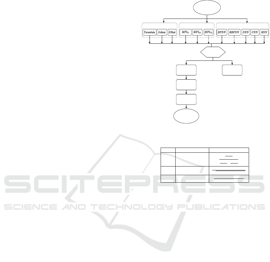
the statements. Figure 1 shows the ﬂow diagram of

our proposed EBFL technique. EBFL takes program

spectra and test execution results as inputs and gener-

ates a ranked list of statements as output.

2.1 Spectrum Based Fault Localization

In SBFL techniques, invocation information of pro-

gram elements and execution results for a number of

Program Spectra and Test

Execution Results

SBFL MBFL NNBFL

Voting to classify

statements

Suspicious

Statements

Non-Suspicious

Statements

Score

Normalization

Combining scores

with Learning to

Rank

Prioritized list of

suspicious statements

Figure 1: Flow diagram of EBFL.

Table 1: SBFL techniques and their formulas.

S.No. SBFL Technique Formula

1 Tarantula

e f

(s)

e f

(s)

2 Ochiai

e f

(s)

√

)×(N

e f

(s)+N

(s))

3 DStar(D

∗

)

e f

(s))

∗

(s))×(N

−N

e f

(s))

test cases are used as input. With these information,

suspiciousness scores of program elements are com-

puted using a mathematical formula. We now brieﬂy

review the important SBFL techniques that have been

proposed by researchers.

Tarantula(Jones et al., 2002): Tarantula is consid-

ered to be a classic SBFL technique. It was introduced

based on the fact that the statements mainly invoked

by failed test cases are more susceptible to contain a

bug as compared to the statements that are invoked by

mainly passed test cases.

Ochiai(Abreu et al., 2007): Ochiai was motivated

from molecular biology ﬁeld. Other SBFL techniques

e.g., Ample (Wong et al., 2016), Jaccard (Wong et al.,

2010), etc. uses only the information in failed and

passed runs. Whereas, Ochiai also considers the count

of failed test cases which have not executed the state-

ment while computing suspiciousness value.

DStar (D

∗

) (Wong et al., 2013): DStar uses a mod-

iﬁed form of the Kulczynski coefﬁcient (Choi et al.,

2010). It assigns suspiciousness value to a statement

directly proportional to the number of failed tests that

executed it. Table 1 shows the formulas used to cal-

culate suspiciousness score using SBFL techniques.

ICSOFT 2022 - 17th International Conference on Software Technologies

160

Table 2: Symbols used in SBFL techniques in Table 1.

Notation Meaning

# passed test cases present

# failed test cases present

(s) # passed test cases invoked statement s

e f

(s) # failed test cases invoked statement s

Table 3: MBFL techniques and their formulas.

MBFL Technique Abbv. Formula

M-FL with Tarantula MFL

max

m∈M(s)

(

k f

(s)

e f

(s)

)

M-FL with Ochiai MFL

max

m∈M(s)

(

k f

(s)

√

)×(N

k f

(s)+N

(s))

)

M-FL with DStar(D

∗

) MFL

max

m∈M(s)

(

k f

(s))

∗

(s))×(N

−N

k f

(s))

)

Table 4: Symbols used in MBFL techniques in Table 3.

Notation Meaning

M(s) Set of mutants created for statement s

m A mutant from set M(s)

(s) Total passed test cases killed by mutant m

k f

(s) Total failed test cases killed by mutant m

2.2 Mutation Based Fault Localization

Though SBFL techniques have been intensively stud-

ied but they have limitations. Key reason is that many

times a fault-free statement is executed by all the

failed test cases and also passed test cases may exe-

cute the faulty statement coincidentally. To mitigate

this problem, MBFL was introduced. In MBFL tech-

niques, a number of mutants for each statement are

created. Based on these, FL is done. We brieﬂy re-

view an important MBFL technique in the following.

Metallaxis-FL (Papadakis and Le Traon, 2015): It is

a well-known MBFL technique and has been reported

to outperform many prominent SBFL techniques. Pa-

padakis et al. map the statement coverage informa-

tion used in SBFL techniques with the number of

pass and fail test cases that kill a mutant. Subse-

quently, they used an SBFL formula to compute the

suspiciousness score of a statement. In EBFL, we use

the same formulas as Tarantula, Ochiai, and D

∗

with

Metallaxis-FL to generate the suspiciousness scores

of the statements. Table 3 shows the formulas used

to calculate the suspuciousness score of a statement

using Metallaxis-FL.

2.3 Neural Network Based Fault

Localization

MBFL techniques are effective, but their effectiveness

gets considerably reduced either when all or none of

the mutants are killed by the failed test cases. Another

drawback of these techniques is that, they are com-

pute intensive. Neural network models can be used

to minimize these limitations. Statement coverage in-

formation along with the test results have been con-

sidered as training samples and labels of training data

respectively for NN models. Subsequently, a virtual

test suite is used to test the trained model and com-

pute the suspiciousness scores of each statement. We

use ﬁve representative neural network models in our

ensemble classiﬁer EBFL.

BPNN-FL (Duda and Hart, 1973): Back propaga-

tion neural network (BPNN) is the simplest and eas-

iest to implement. We use the same architecture as

discussed by Wong et al.(Wong and Qi, 2009).

RBFNN-FL (Mitchell et al., 1997): RBFNN easily

maps the complex functions and free from the prob-

lems like local minima(Duda and Hart, 1973) and

paralysis (Wasserman, 1993). The RBFNN model

used in EBFL is as same as in (Wong et al., 2011).

DNN-FL (Mitchell et al., 1997): DNNs are pow-

erful enough to correctly approximate considerably

complex functions. It achieves this by the distributed

representation for input data which can be learnt by

the non-linear network structures in presence of lim-

ited samples also. Other than the input and output

layers, three hidden layers are present in the DNN

model that we use. Other optimizations and network

settings used in DNN are the as same as in (Zheng

et al., 2016).

CNN-FL (Ketkar, 2017): Convolutional neural net-

work (CNN) is an important class of deep neural net-

works. It can efﬁciently work with large-sized data

sets using its parameter sharing and down sampling

features. Also, CNNs have good generalization capa-

bility. In the CNN model which we have used, there

are two convolutional layers, two pooling layers, and

two rectiﬁed linear units (ReLu) to connect the con-

volutional layer and pooling layer. A fully connected

three layered NN has been discussed subsequently.

RNN-FL (Sherstinsky, 2020): Another popular deep

neural network architecture is recurrent neural net-

work (RNN). RNNs have memory which stores pre-

viously computed information. RNN uses same pa-

rameters for each of the inputs on which it has per-

form the similar functions on all hidden as well as

input layers to generate the output. RNN model used

in EBFL contains one input, three recurrent and one

output layers in complete.

2.4 Ensemble Classiﬁer Based Fault

Localization (EBFL)

We ﬁrst generate the suspiciousness scores of all

statements using each FL technique considered. Fur-

ther, the medians of the suspiciousness scores gen-

An Ensemble Classiﬁer based Method for Effective Fault Localization

161

erated by each technique are computed. We apply a

voting strategy to classify the program statements into

two classes viz., non-suspicious and suspicious. Ac-

cording to our voting strategy, if a statement’s suspi-

ciousness scores for six or above number of FL tech-

niques, are higher than or equal to that particular FL

technique’s median value, then the statement is con-

sidered into the suspicious class otherwise it is con-

sidered into the non-suspicious class.

After separating the statements into two classes,

we normalize the suspiciousness scores generated by

different techniques. Suspiciousness scores generated

by RBFNN, BPNN and Tarantula are always between

0 to 1, whereas, DStar generates scores any positive

values. We then normalize the suspiciousness val-

ues generated by all the FL techniques in range of

0 to 1 to maintain a uniformity among all the tech-

niques. To achieve this, the suspicious value of each

statement is divided by the summation of the suspi-

ciousness scores of all the statements for the respec-

tive FL technique.

Subsequently, we combine the suspiciousness

scores generated by all the FL techniques to assign

a single suspiciousness score to a statement. We

use learning to rank algorithm (Xuan and Monper-

rus, 2014) to add weights to each FL technique. The

combined suspiciousness score of statement e is cal-

culated using Equation 1.

susp(e) =

∑

i=1

(e) ∗ss

(e) (1)

where, w

(e) and ss

(e) denote the weight of the i

FL technique and suspiciousness score for statement

e generated by the same FL technique respectively.

Learning-to-Rank algorithm learns the order be-

tween non-faulty and faulty statements such that the

faulty statements always have higher suspiciousness

score than the non-faulty ones. The loss function used

by the algorithm is given in Equation 2.

loss =

∑

−

||susp(e

) ≤ susp(e

−

)|| (2)

Where, < e

, e

−

> denotes a pair of faulty and cor-

rect statements and loss function computes the num-

ber of pairs for which the suspiciousness score of

faulty statement is less than the correct statements.

The input data required for learning-to-rank (LTR)

algorithm is given in Table 5. In the table, Column

1 (SID) shows the statement number and and Column

2 (VID) shows the version number of faulty program

considered. Column 3 (FT) represents whether the

statement is faulty or not. If it contains ‘1’, then the

statement of that version is faulty otherwise not. Re-

maining columns contains the suspiciousness scores

Table 5: Sample training data for LTR algorithm.

SID VID FT Susp

Susp

···

1 0 SS

(1,1)

···

2 1 SS

(1,2)

···

1 0 SS

(2,1)

···

2 0 SS

(2,2)

···

··· ··· ··· ··· ··· ··· ···

generated by different FL techniques. For exam-

ple, SS

(1,2)

contains the suspiciousness score gener-

ated by FL technique 3 for the 1

statement of 2

faulty version. Different pairwise Learning-to-Rank

approaches can be applied for fault localization, e.g.,

RankBoost, RankNet and FRank etc. We have used

RankBoost algorithm in EBFL. RankBoost (Freund

et al., 1998) is classic and efﬁcient approach based on

Adaboost.

2.5 Multiple Fault Localization

Till now we have discussed our localization method

for single-fault programs. However, in practice, a pro-

gram may contain multiple faults. We extend our pro-

posed technique Combi-FL to handle multiple-fault

programs using the concept of parallel debugging

(Jones et al., 2007). For parallel debugging, failed

test cases are divided into different fault focused clus-

ters. Subsequently, each of these clusters is used to lo-

calized the bugs in parallel. These steps are repeated

until all the test cases are pass.

2.5.1 Creation of Fault-focused Cluster

Let us consider that there are p

and f

number of

unique pass and unique failed test cases are present

in the test suite. Here, the term ‘unique’ stands in

terms of unique statement coverage vectors. Initially,

we create f

number of test suites by combining one

failed test case with all the p

test cases. Subse-

quently, we apply the EBFL technique over each of

the f

test suites to generate f

statement ranking se-

quences corresponding to each failed test case vector.

We further compute the similarity among different

statement ranking sequences using revised Kendall’s

tau correlation coefﬁcient deﬁned by Gao et al. (Gao

and Wong, 2017). In revised Kendall’s tau coefﬁ-

cient (Knight, 1966) computation, high weights are

assigned to the statements holding higher ranks and

low weights to the lower ranking statements. The ob-

tained ranking sequences are combined based on their

similarity using the agglomerative hierarchical clus-

tering method (Davidson and Ravi, 2005). This pro-

cess continues until a single cluster formed. It results

in a f

-level hierarchical tree.

ICSOFT 2022 - 17th International Conference on Software Technologies

162

2.5.2 Stopping Criterion

Our stopping criterion is based on a measure the simi-

larity between the top-25% of ranking sequences gen-

erated by the clusters present at the k

and (k −1)

levels of the hierarchical tree. We use Jaccard simi-

larity metric to compute the similarity between rank-

ing sequences. If the Jaccard similarity is more than

85%, we consider the faulty location indicated by the

test cluster at k

and (k −1)

levels are same. On the

other hand, if the similarity score is less than 85%,

then the buggy locations indicated are different and

clusters are further broken up to ﬁnd the correct loca-

tion. This process is repeated until all the bugs have

been located in the code.

3 EXPERIMENTAL RESULTS

In this section, we present the used setup and pro-

grams for our experiments. Followed by this, we

discuss the obtained experimental results. The sec-

tion is completed by discussing some of the important

threats to the validity of experimental results.

3.1 Setup

The experiments were performed on a 64-bit Ubuntu

machine with 16 Giga Bytes RAM and Intel core

processor. The input C-programs are complied us-

ing GCC-7.4.0 compiler. Information of program

spectra and test execution results were obtained us-

ing GCOV(gcov, 2002) tool. Since, Defects4j pro-

gram suite contains Java programs, we used open-

source available coverage results and other required

resources in our experiment are taken from (De-

fects4J, 2014). We have developed a mutator to create

the mutants and it is available online (Mutator, 2019)

for use.

3.2 Subject Programs

To evaluate the effectiveness of EBFL, we have ex-

perimented with four program suites comprising of

eleven different programs. We have used three bench-

mark suites: Siemens suite, Space

2.0, and Gzip 1.50

downloaded from SIR repository(SIR, 2005). Last

two programs are taken from Defects4j (Defects4J,

2014). The benchmark program suites also accompa-

nied by faulty versions and test cases. Table 6 shows

some of the important characteristics of the programs

used in our experimental study. Columns 2-5 present

the program name, number of faulty versions, number

of executable statements, total number of test cases

Figure 2: Effectiveness of EBFL, D

∗

and Tarantula for the

Siemens suite.

and number of mutants generated respectively. For

the last two programs, we have used the statement

coverage information and test execution results al-

ready available in their respective website (Defects4J,

2014).

3.3 Results

We compare the results of EBFL with two SBFL

techniques: Tarantula (Jones et al., 2002) and DStar

(Wong et al., 2013) and two NNBFL techniques:

DNN(Zheng et al., 2016) and CNN(Zhang et al.,

2019). Since, SBFL techniques sometimes allot the

same suspiciousness value to two or more number

of program statements, which leads to two different

types of effectiveness, the worst effectiveness and the

best effectiveness. On the other hand, EBFL, CNN

(Zhang et al., 2019), and DNN (Zheng et al., 2016) as-

sign unique suspiciousness scores to each statement.

For this reason, in the line graphs 2 to 7, the effective-

ness of SBFL techniques are represented with two dif-

ferent line plots and other techniques are represented

with a single line plot.

Table 6: Program characteristics.

Program No. of No. of No. of No. of

Name Flty. Ver. Ex. LOC Tests Mutants

Print Tokens 7 195 4130 285

Print Tokens2 10 200 4115 314

Schedule 9 152 2650 406

Schedule2 10 128 2710 350

Replace 32 244 5542 508

Tcas 41 65 1608 216

Tot info 23 122 1052 571

Space 2.0 38 3656 13585 17521

Gzip 1.50 13 1720 195 8250

Time 27 40.1K 4130 416

Lang 65 30.2K 2245 775

Figure 2 represents the effectiveness comparison

of EBFL, DStar and Tarantula for the Siemens suite

programs. It can be observed from the ﬁgure that

An Ensemble Classiﬁer based Method for Effective Fault Localization

163

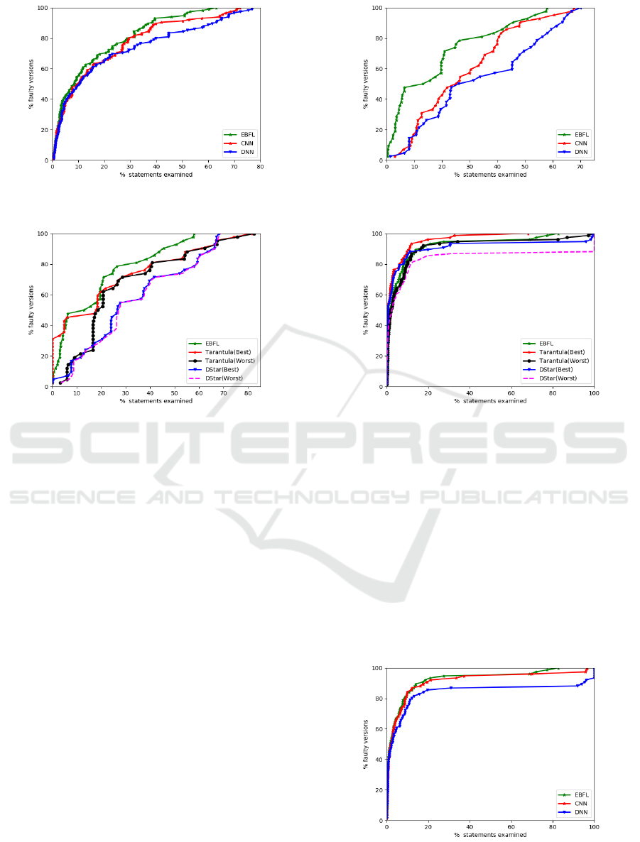
Figure 3: Effectiveness of EBFL, CNN and DNN for the

Siemens suite.

Figure 4: Effectiveness of EBFL, D

∗

and Tarantula for Gzip

and Space.

by examining 10% of statements, Tarantula(Best)

and Tarantula(Worst), and DStar(Worst) localize bugs

in 46.08%, 39.13%, and 45.21% of faulty versions.

Whereas, by examining the same percentage of state-

ments, EBFL localized bugs in 58.48% of faulty pro-

grams. On an average, when using EBFL it is neces-

sary to examine 20.44% and 35.50% less statements

than DStar and Tarantula respectively.

Figure 3 shows the experimental results of EBFL,

CNN, and DNN for the Siemens suite. It can be ob-

served that EBFL outperforms both CNN and DNN.

In the worst case, EBFL requires 3% and 6% less code

analysis than CNN and DNN. On an average, EBFL

performs 16.53% and 28.73% more effectively than

both CNN and DNN models respectively for fault lo-

calization.

Figure 4 presents the effectiveness comparison of

EBFL, DStar and Tarantula for the Gzip and Space

suites. We can observe from the line graphs in Fig. 4

that by analysing only 12% of program code, faults

are localized in 50% of faulty versions by EBFL.

However, with the same amount of code analysis,

faults are localized in only 45.23%, 21.42%, 21.42%,

and 19.04% of faulty programs by Tarantula(Best),

Tarantula(Worst), DStar(Best), and DStar(Worst) re-

spectively. Moreover, in the worst case, EBFL is

Figure 5: Effectiveness of EBFL, CNN and DNN for Gzip

and Space.

Figure 6: Effectiveness of EBFL, D

∗

and Tarantula for De-

fects4j.

24.62% and 10.92% better than Tarantula(Best) and

DStar(Best). Therefore, for the Space and Grep suites

of programs, EBFL is, on an average, 46.70% and

25.56% better than DStar and Tarantula respectively.

Figure 5 shows performance results for EBFL,

DNN, and CNN using the Gzip and Space programs.

We can observe from the ﬁgure 5 that for almost all

the faulty programs, EBFL performs more effectively

than both DNN and CNN. By analysing only 10% of

the program code, EBFL localizes bugs in 47.61%

of faulty versions whereas, DNN and CNN localize

bugs in only in 16.67% and 19.04% of versions for

Figure 7: Effectiveness of EBFL, CNN and DNN for De-

fects4j.

ICSOFT 2022 - 17th International Conference on Software Technologies

164

Table 7: Relative improvement using EBFL over existing

FL techniques.

Programs Tarantula DStar DNN CNN

Siemens 64.59 79.59 71.29 83.50

Space 69.74 49.87 49.37 60.61

Gzip 85.01 76.11 83.83 89.06

Defects4j 87.05 58.82 47.12 85.15

the same amount of code examination. Further, in

the worst case, EBFL performs 12.22% and 9.88%

more effectively than DNN and CNN respectively. On

an average, EBFL examines respectively 47.36% and

35.03% less code than DNN and CNN.

Figure 6 presents the effectiveness comparison of

EBFL, DStar and Tarantula for the Defects4j pro-

grams. We can observe from the ﬁgure that by exam-

ining only 1% of program code EBFL localizes faults

in 44.73% of buggy versions of Defects4j. Whereas,

Tarantula(Worst), and DStar(Worst) require to exam-

ine at least 1.36%, and 1.53% of code. In the worst

case, EBFL is 33.69% better than DStar and Taran-

tula. EBFL is, on an average, 8.63% and 39.62%

more effective than Tarantula and DStar respectively.

Figure 7 shows effectiveness comparison of re-

sults of EBFL, DNN, and CNN for Defects4j pro-

gram suite. By checking 0.03% of program code,

EBFL localizes bugs in 23.68% of the faulty ver-

sion. Whereas, with the same EXAM

Score, CNN

and DNN are able to localize bugs in only 18.42%

and 17.10% of faulty program versions respectively.

EBFL is, on an average, 60.68% more effective than

DNN; and 28.93% more effective than CNN in local-

izing software faults.

Table 7 shows the relative improvement achieved

using EBFL over the existing FL techniques. It can

be observed that for almost all the considered pro-

grams, EBFL performs better than Tarantula, DStar,

DNN and CNN.

3.4 Threats to Validity

We present a few important threats to the validity of

our obtained experimental results.

• We have experimented our EBFL approach over

limited set of programs. It may possible that the

results are not similar for other set of programs.

However, to mitigate this risk, we have examined

program from different application domains and

variable complexities, LOCs etc.

• Effectiveness of EBFL technique lies on proper

combination of passed and failed test cases. If the

test suite is biased, for example, either all the test

cases are passed or failed, then it will not perform

effectively.

4 COMPARISON WITH

RELATED WORK

We have experimentally compared our proposed

EBFL technique with two prominent SBFL tech-

niques: DStar (Wong et al., 2013), and Tarantula

(Jones et al., 2002). Our results indicate that EBFL

performs, on an average, 37.88%, and 25.43% bet-

ter than DStar and Tarantula respectively for the con-

sidered programs. Also, EBFL assigns a unique sus-

piciousness score to each statements. This is unlike

SBFL techniques which may assign the same suspi-

ciousness scores to two or more statements.

Different slicing based fault localization tech-

niques have been proposed and reported (Agrawal

and Horgan, 1990; Lyle, 1987; Weiser, 1984). These

techniques yields a set of suspected statements only.

They do not assign any ranking to the statements even

which hampers the effectiveness of a FL technique.

Also, sometimes a slice may contain all or most of

the statements present in the program. On the other

hand, EBFL assigns unique suspiciousness values to

each of the executable statement present in the suspi-

cious class.

Renieris et al. (Renieres and Reiss, 2003) pro-

posed a FL technique based nearest neighbor con-

cept. This technique discovers the most similar ex-

ecution trace covered by a failed test case with that

covered by different passed test cases. Subsequently,

they have used set difference to remove the irrele-

vant statements and reports the suspicious set of state-

ments. Their approach sometimes returns a empty

set of suspicious statements too. Whereas, EBFL

ﬁrst classiﬁes the statements into two separate groups:

non-suspicious and suspicious using a voting-scheme

based on the suspiciousness scores generated by dif-

ferent techniques. Our proposed EBFL method will

never return an empty set of suspicious statements.

Xuan et al. (Xuan and Monperrus, 2014) pro-

posed a technique to merge different spectrum based

fault localization methods using learning-to-rank al-

gorithm to generate effective prioritized list of state-

ments. On the other hand, in EBFL, we have consid-

ered three different domains of fault localization tech-

niques: spectrum based, mutation based and neural

network techniques for better localization of faults.

5 CONCLUSION

Fault localization is an important part of debugging.

To make bug localization easier and effective, we

have proposed an ensemble classiﬁer based tech-

nique. We have combined three different families of

An Ensemble Classiﬁer based Method for Effective Fault Localization

165

FL techniques viz., SBFL, MBFL, and NNBFL. Our

method is able to effectively localize common as well

as instrinsic bugs present in the program. Empirical

evaluation shows that, on an average, EBFL performs

58% more effectively in terms of less code examina-

tion than cntemporary FL techniques.

In future, we make use of the individual bug ex-

posing capabilities of test cases to improve the effec-

tiveness of EBFL.

REFERENCES

Abreu, R., Zoeteweij, P., and Van Gemund, A. J. (2007). On

the accuracy of spectrum-based fault localization. In

TAICPART-MUTATION 2007, pages 89–98.

Agrawal, H. and Horgan, J. R. (1990). Dynamic program

slicing. ACM SIGPlan Notices, 25(6):246–256.

Choi, S.-S., Cha, S.-H., and Tappert, C. C. (2010). A survey

of binary similarity and distance measures. Journal of

Systemics, Cybernetics and Informatics, 8(1):43–48.

Davidson, I. and Ravi, S. (2005). Agglomerative hierarchi-

cal clustering with constraints: Theoretical and empir-

ical results. In European Conference on Principles of

Data Mining and Knowledge Discovery, pages 59–70.

Defects4J (2014). github.com/rjust/defects4j.

Duda, R. O. and Hart, P. E. (1973). Pattern recognition and

scene analysis.

Dutta, A., Kunal, K., Srivastava, S. S., Shankar, S., and

Mall, R. (2021). Ftﬂ: A ﬁsher’s test-based approach

for fault localization. Innovations in Systems and Soft-

ware Engineering, pages 1–25.

Dutta, A., Manral, R., Mitra, P., and Mall, R. (2019a). Hier-

archically localizing software faults using dnn. IEEE

Transactions on Reliability, 69(4):1267–1292.

Dutta, A., Pant, N., Mitra, P., and Mall, R. (2019b). Effec-

tive fault localization using an ensemble classiﬁer. In

QR2MSE, pages 847–855. IEEE.

Freund, Y., Iyer, R., Schapire, R. E., and Singer, Y. (1998).

An e cient boosting algorithm for combining prefer-

ences. In ICML. Citeseer.

Gao, R. and Wong, W. E. (2017). Mseer—an advanced

technique for locating multiple bugs in parallel. IEEE

Transactions on Software Engineering, 45(3):301–

318.

gcov (2002). man7.org/linux/man-pages/man1/gcov-tool.

1.html.

Jones, J. A., Bowring, J. F., and Harrold, M. J. (2007). De-

bugging in parallel. In Proceedings of the 2007 inter-

national symposium on Software testing and analysis,

pages 16–26.

Jones, J. A., Harrold, M. J., and Stasko, J. (2002). Visual-

ization of test information to assist fault localization.

In ICSE, pages 467–477. IEEE.

Ketkar, N. (2017). Convolutional neural networks. In Deep

Learning with Python, pages 63–78. Springer.

Knight, W. R. (1966). A computer method for calculat-

ing kendall’s tau with ungrouped data. Journal of the

American Statistical Association, 61(314):436–439.

Krinke, J. (2004). Slicing, chopping, and path conditions

with barriers. Software Quality Journal, 12(4).

Lyle, R. (1987). Automatic program bug location by pro-

gram slicing. In 2nd international conference on com-

puters and applications, pages 877–883.

Mitchell, T. M. et al. (1997). Machine learning.

Moon, S., Kim, Y., Kim, M., and Yoo, S. (2014). Ask the

mutants: Mutating faulty programs for fault localiza-

tion. In 7th STVV, pages 153–162.

Mutator (2019). github.com/ArpitaDutta/Mutator .

Papadakis, M. and Le Traon, Y. (2015). Metallaxis-

ﬂ: mutation-based fault localization. STVR, 25(5-

7):605–628.

Renieres, M. and Reiss, S. P. (2003). Fault localization with

nearest neighbor queries. In 18th ASE, pages 30–39.

Sherstinsky, A. (2020). Fundamentals of rnn and

lstm network. Physica D: Nonlinear Phenomena,

404:132306.

SIR (2005). sir.unl.edu/portal/index.php.

Sridharan, M., Fink, S. J., and Bodik, R. (2007). Thin slic-

ing. In 28th PLDI, pages 112–122.

Wasserman, P. D. (1993). Advanced methods in neural com-

puting. John Wiley & Sons, Inc.

Weiser, M. (1984). Program slicing. IEEE Transactions on

software engineering, (4):352–357.

Wong, W. E., Debroy, V., and Choi, B. (2010). A family

of code coverage-based heuristics for effective fault

localization. JSS, 83(2):188–208.

Wong, W. E., Debroy, V., Gao, R., and Li, Y. (2013). The

dstar method for effective software fault localization.

IEEE Transactions on Reliability, 63(1):290–308.

Wong, W. E., Debroy, V., Golden, R., Xu, X., and Thurais-

ingham, B. (2011). Effective software fault localiza-

tion using an rbf neural network. IEEE Transactions

on Reliability, 61(1):149–169.

Wong, W. E., Gao, R., Li, Y., Abreu, R., and Wotawa, F.

(2016). A survey on software fault localization. IEEE

TSE, 42(8):707–740.

Wong, W. E. and Qi, Y. (2009). Bp neural network-based

effective fault localization. IJSEKE, 19(04):573–597.

Xuan, J. and Monperrus, M. (2014). Learning to combine

multiple ranking metrics for fault localization. In 2014

IEEE ICMSE, pages 191–200.

Zhang, Z., Lei, Y., Mao, X., and Li, P. (2019). Cnn-ﬂ: An

effective approach for localizing faults using convolu-

tional neural networks. In SANER, pages 445–455.

Zhang, Z., Lei, Y., Tan, Q., Mao, X., Zeng, P., and Chang,

X. (2017). Deep learning-based fault localization with

contextual information. IEICE Transactions on Infor-

mation and Systems, 100(12):3027–3031.

Zheng, W., Hu, D., and Wang, J. (2016). Fault localization

analysis based on deep neural network. Mathematical

Problems in Engineering.

ICSOFT 2022 - 17th International Conference on Software Technologies

166