
Generalized Mutant Subsumption
Samia Al Blwi
1
, Imen Marsit
2
, Besma Khaireddine
3
, Amani Ayad
4
, JiMeng Loh
1
and Ali Mili
1
a
1
NJIT, Newark, NJ, U.S.A.
2
University of Sousse, Sousse, Tunisia
3
University of Tunis El Manar, Tunis, Tunisia
4
Kean University, Union, NJ, U.S.A.
mili@njit.edu
Keywords:
Mutation Testing, Mutant Subsumption, Differentiator Sets.
Abstract:
Mutant Subsumption is an ordering relation between the mutants of a base program, which ranks mutants
according to inclusion relationships between their differentiator sets. The differentiator set of a mutant with
respect to a base program is the set of inputs for which execution of the base program and the mutant produce
different outcomes. In this paper we propose to refine the definition of mutant subsumption by pondering, in
turn: what do we consider to be the outcome of a program’s execution? under what condition do we consider
that two outcomes are comparable? and under what condition do we consider that two comparable outcomes
are identical? We find that the way we answer these questions determines what it means to kill a mutant, how
subsumption is defined, how mutants are ordered by subsumption, and what set of mutants is minimal.
1 INTRODUCTION
1.1 Program Executions and Outcomes
The mutants of a program are generated by applying
localized syntactic alterations to the source code of a
program, and are typically used to assess the quality
of test suites: a good test suite is one that yields dif-
ferent outcomes (from the base program) for all the
mutants that are not semantically equivalent to the
program. Mutation testing is a reliable way to as-
sess the effectiveness of test suites, but it is also an
expensive proposition. As a consequence, it is sen-
sible to try to reduce the size of mutant sets, without
loss of effectiveness. In (Marsit et al., 2021), Mar-
sit et al. propose an algorithm to reduce the size of a
set of mutants by partitionning the set of mutants into
equivalence classes, modulo semantic equivalence,
and retaining one mutant from each equivalence class.
While this criterion is non-controversial (two seman-
tically equivalent mutants are as good as just one), it
may be sub-optimal: In (Guimaraes et al., 2020; Par-
sai and Demeyer, 2017; Souza, 2020; Li et al., 2017;
Jia and Harman, 2008; Kurtz et al., 2014; Kurtz et al.,
2015; Tenorio et al., 2019), a more sophisticated cri-
a
https://orcid.org/0000-0002-6578-5510
terion is used: a partial ordering is defined between
mutants of a given base program P, whereby a mutant
M is said to subsume a mutant M
′
if and only if M
produces a different outcome from P for at least one
input, and any input for which M produces a different
outcome from P, M
′
produces necessarily a different
outcome from P.
The original definition of mutant subsumption
(Kurtz et al., 2014) refers to program outcomes be-
ing identical or distinct, but does not dwell on what
exactly is the outcome of a program and when can
we consider that two program outcomes are identical.
In this paper we propose to generalize the concept of
subsumption by seeking to ponder the following ques-
tions:
• What Is the Outcome of a Program? Programs
and mutants do not always terminate normally and
produce a well-defined/ agreed upon outcome.
Programs may fail to terminate (if they enter an
infinite loop, and eventually time out), or they
may encounter an exceptional condition, such as
an array reference out of bounds, a reference to
a nil pointer, a division by zero, an undefined ex-
pression (e.g. the logarithm of a negative num-
ber), an overflow, an underflow, etc. In fact many
mutation operators are prone to create the condi-
tions of divergence even when the original pro-
46
Al Blwi, S., Marsit, I., Khaireddine, B., Ayad, A., Loh, J. and Mili, A.
Generalized Mutant Subsumption.
DOI: 10.5220/0011166700003266
In Proceedings of the 17th International Conference on Software Technologies (ICSOFT 2022), pages 46-56
ISBN: 978-989-758-588-3; ISSN: 2184-2833
Copyright
c
2022 by SCITEPRESS – Science and Technology Publications, Lda. All rights reserved

gram terminates normally. The question that we
must ponder is: when a program fails to converge,
do we consider that it has no outcome, or that fail-
ure to converge is itself an outcome.
Also, even when a program does terminate nor-
mally, it is not always clear what we consider to
be its outcome: is it its final state or the output
that the program delivers as a projection of the
final state? For example, if a program permutes
two variables x and y using an auxiliary variable
z, what is the outcome of the program? is it the
final values of x, y and z, or just the final values of
x and y? This can get more complicated/ ambigu-
ous when we consider global variables, parame-
ter passing, communication channels, operations
with side effects, etc.
• Under what condition do we consider that the
Outcomes of Two Programs Are Comparable?
When the execution of a program on some input
terminates after a finite number of steps without
causing any exception, such as an array reference
out of bounds, a reference to a nil pointer, a run-
time stack overflow, or an illegal operation (such
as a square root of a negative number, the log of
zero or a negative number, a division by zero, an
arithmetic overflow, etc) we say that the execu-
tion converges (or: terminates normally); else we
say that the execution diverges. When two pro-
grams converge, comparing their outcomes poses
no problem; but we must decide whether their out-
comes are comparbale when one of them or both
of them diverge.
• When Do We Consider That Two Program Out-
comes Are Identical or Distinct? If we consider
that the outcome of a program that converges and
the outcome of a program that diverges are com-
parable, then it is sensible to consider that their
outcomes are distinct. But if two programs di-
verge for a given input, do we consider that their
outcomes are incomparable, or that they are com-
parable and identical? What if the divergence is of
the same type (e.g. both fail to terminate, or both
attempt a division by zero, etc)? What if both fails
at the same statement of the source code?
In this paper we argue that the definition of subsump-
tion depends critically on how we answer these three
questions. Specifically, we present three possible def-
initions of subsumption, which correspond to differ-
ent interpretations of program outcomes and how to
compare them. Then we show on a concrete exam-
ple how these yield different ordering relations on the
mutants of a base program, and different minimal mu-
tant sets. It appears that the original definition of mu-
tant subsumption (Kurtz et al., 2014) makes no provi-
sion for the possibility of divergence, hence assumes
implicitly that programs and mutants converge for all
inputs; it also seems to assume that the outcome of
a program that converges is well-understood, hence
requires no careful consideration.
1.2 Motivation
While the discussion of what is a program outcome
and when two program outcomes are considered iden-
tical may sound like an academic exercise in hair-
splitting, we argue that it is fact an important con-
sideration in mutation testing, because many muta-
tion operators are prone to cause programs to diverge,
even when the base program converges:
• if we consider a loop that addresses an array at
indices 0 through N − 1
while (i<N)
{
a[i]=..;...;i++;
}
and the logical operator
<
is changed to
<=
then
the resulting mutant will diverge due to an array
index out of bound.
• If we consider a guarded assignment statement
such as:
if ((x!=0) && (x!=1))
{
y=1/x(x-1);
}
and the
&&
is replaced by a logical OR
||
, then
the resulting mutant will diverge for x = 0 and for
x = 1, due to a division by zero.
• If we consider a loop that decrements an integer
variable by 2 at each iteration while the variable
is positive,
x=5; while (x>0)
{
x=x-2;..;
}
and we change the comparison operator
>
to
!=
,
then (if the initial value is odd) the resulting mu-
tant will diverge due to an infinite loop.
In theory, we should also consider cases where the
base program itself may fail to converge for some test
data; of course one may wonder why we would test
a program outside its domain, but it is the domain of
the specification, not the domain of the program, that
determines what test data to run.
1.3 Agenda
To discuss these questions, we need to introduce a
framework for defining and analyzing program func-
tions; this is the subject of section 2. In section 3
we introduce the concept of differentiator set, which
serves as a basis for redefining subsumption, and in
section 4 we present three distinct definitions of sub-
sumption. In section 5 we consider a benchmark pro-
gram, generate its mutants, then we analyze subsump-
tion relationships between these mutants, using the
Generalized Mutant Subsumption
47

three definitions introduced in section 4; we show that
(not surprisingly) these three definitions give three
distinct subsumption graphs, and three distinct min-
imal mutant sets. In section 6 we summarize our find-
ings and suggest venues for further investigation.
2 MATHEMATICS FOR
PROGRAM ANALYSIS
2.1 Sets and Relations
In this paper, we use relations and functions (Brink
et al., 1997; Schmidt, 2010) to capture program spec-
ifications and program semantics. For the sake of sim-
plicity, and without loss of generality, we consider ho-
mogeneous relations on sets represented by program-
like declarations. Modeling the program behavior by
homogeneous relations encompasses the case where
we want to model it by a relation from inputs to out-
puts: it suffices to add an input stream and an output
stream as state variables. We generally denote sets
(referred to as spaces) by S, elements of S (referred to
as states) by lower case s, specifications (binary rela-
tions on S) by R and programs (functions on S) by P,
Q. We denote the domain of a relation R (or a func-
tion P) by dom(R) (dom(P)). Because we model pro-
grams and specifications by homogeneous relations /
functions, we usually talk about initial states and final
states; we may talk about inputs to refer to the initial
value of the input stream and outputs to refer to the
final value of the output stream.
2.2 Programs and Specifications
A specification R includes all the initial state / final
state pairs that the specifier considers correct; hence
the domain of a specification R (dom(R)) includes all
the initial states for which candidate programs must
make provisions. A program P includes all the ini-
tial state/ final state pairs (s, s
′
) such that if P starts
execution in initial state s it terminates normally (i.e.
after a finite number of steps, without raising an ex-
ception) in state s
′
. From this definition, it stems that
the domain of program P (dom(P)) is the set of initial
states s such that execution of P on s terminates after
a finite number of steps, and does not raise an excep-
tion (such as an overflow, underflow, division by zero,
array reference out of bounds, etc).
For the sake of simplicity, we restrict our study
to deterministic programs, i.e. programs which map
each initial state to at most one final state. It would be
interesting to include non-deterministic programs (in-
cluding concurrent programs), but this would compli-
cate our model, and introduce other mutation-specific
difficulties (Vercammen et al., 2021).
2.3 Absolute Correctness
We consider a program P on space S and a specifica-
tion R on S; without loss of generality, we model the
semantics of a program by the (homogeneous) rela-
tion that the program defines from its initial states to
its final states.
Definition 1. We say that a program P on space S is
correct with respect to specification R on S if and only
if:
dom(R) = dom(R∩ P).
Intuitively, a program P is correct with respect to
a specification R if and only if for all s in dom(R), ex-
ecution of P on s converges and produces a final state
that satisfies the condition (s, P(s)) ∈ R. The domain
of the intersection of R and P represents the set of
initial states for which program P behaves as R man-
dates; it is called the competence domain of P with
respect to R. Figure 1 shows a simple example of a
(non-deterministic) specification R and two programs
P and P
′
such that P is correct with respect to R and P
′
is not; the competence domains of P and P
′
are shown
by the ovals.
Definition 2. We say that a program P on space S is
partially correct with respect to specification R on S if
and only if:
dom(R) ∩ dom(P) = dom(R∩ P).
Intuitively, a program P is partially correct with
respect to a specification R if and only if for all s
in dom(R), if execution of P on s converges then
it produces a final state that satisfies the condition
(s, P(s)) ∈ R. When we want to contrast correct-
ness with partial correctness, we may refer to the for-
mer as total correctness. Our definitions of total and
partial correctness are equivalent, modulo differences
of notation, to traditional definitions with respect to
pre/post specifications (Hoare, 1969; Gries, 1981; Di-
jkstra, 1976; Manna, 1974). See Figure 2: Program Q
is partially correct with respect to R because for any
initial state of dom(R) for which it terminates, pro-
gram Q delivers a final state that satisfies specifica-
tion R; by contrast, program Q
′
is not partially correct
with respect to R, even though it terminates normally
for all initial states in dom(R), because it does not sat-
isfy specification R; neither Q nor Q
′
is totally correct
with respect to R. We admit without proof that if P is
totally correct with respect to R then it is necessarily
partially correct with respect to R.
ICSOFT 2022 - 17th International Conference on Software Technologies
48

3
2
1
0
3
2
1
0
3
2
1
0
3
2
1
0
3
2
1
0
3
2
1
0
✘
✘
✘
✘
✘
✘✿
❳
❳
❳
❳
❳
❳③
✲
✘
✘
✘
✘
✘
✘✿
❳
❳
❳
❳
❳
❳③
✲
❳
❳
❳
❳
❳
❳③
❳
❳
❳
❳
❳
❳③
❳
❳
❳
❳
❳
❳③
✲
✘
✘
✘
✘
✘
✘✿
✟
✟
✟
✟
✟
✟✯
✚
✚
✚
✚
✚
✚❃
✄
✂
✁
✄
✂
✁
P R
P
′
dom(R ∩ P) = {1, 2}
= dom(R) ⇒ P correct
dom(R∩ P
′
) = {1}
6= dom(R) ⇒ P
′
incorrect
Figure 1: Total Correctness.
3
2
1
0
3
2
1
0
3
2
1
0
3
2
1
0
3
2
1
0
3
2
1
0
✘
✘
✘
✘
✘
✘✿
❳
❳
❳
❳
❳
❳③
✲
✘
✘
✘
✘
✘
✘✿
❳
❳
❳
❳
❳
❳③
✲
✘
✘
✘
✘
✘
✘✿
✘
✘
✘
✘
✘
✘✿
❍
❍
❍
❍
❍
❍❥
✟
✟
✟
✟
✟
✟✯
✄
✂
✁
Q
R
Q
′
dom(R∩ Q) = {1}
= dom(R) ∩ dom(Q)
⇒ Q part. correct
dom(R∩ Q
′
) = {}
6= dom(R) ∩ dom(Q
′
)
⇒ Q
′
not part. correct
Figure 2: Partial Correctness.
2.4 Relative Correctness
Whereas total correctness and partial correctness de-
fine a property between a program and a specifica-
tion, relative correctness defines a property between
two programs and a specification.
Definition 3. Given a specification R on space S and
two programs P and P
′
on S, we say that P
′
is more-
correct than P with respect to R (denoted by: P
′
⊒
R
P
or P ⊑
R
P
′
) if and only if:
dom(R∩ P) ⊆ dom(R∩ P
′
).
In other words, P
′
is more-correct than P with re-
spect to R if and only if it has a larger competence
domain with respect to R. Whenever we want to con-
trast correctness (definition 1) with relative correct-
ness, we may refer to the former as absolute correct-
ness. See Figure 3; it shows two instances of relative
correctness. Q
′
is more-correct than Q by virtue of
imitating the correct behavior of Q; by contrast, P
′
is
more-correct than P by virtue of a differentcorrect be-
havior; because specification R is non-deterministic,
correct behavior is not unique.
3 DIFFERENTIATOR SETS
In section 1, we had argued that while the definitions
of mutant subsumption refer to program outcomes
and to the condition under which two program out-
comes are identical, they are not perfectly clear about
what constitutes the outcome of a program, when
two program outcomes are comparable, and if they
are when can we consider them to be identical. In
this section, we address this ambiguity by introducing
several definitions of differentiator sets, which reflect
different interpretations to the questions above.
Given two programs, say P and Q, the differentia-
tor set of P and Q is the set of initial states for which
execution of P and Q yield different outcomes. For
the purposes of this paper, we adopt the three defini-
tions of differentiator sets proposed by Mili in (Mili,
2021):
• Basic Differentiator Set. The basic differentiator
set of two programs P and Q on space S is defined
only if P and Q converge for all s in S; it is the
set of states s such that P(s) 6= Q(s). This set is
denoted by δ
B
(P, Q) and defined by:
δ
B
(P, Q) =
dom(P∩ Q).
• Strict Differentiator Set. The strict differentiator
set of two programs P and Q on space S is de-
fined regardless of whether P and Q converge for
all initial states. It includes all the states for which
executions of P and Q both converge and yield
distinct outcomes. This set is denoted by δ
S
(P, Q)
and defined by:
δ
S
(P, Q) = dom(P) ∩ dom(Q)∩
dom(P∩ Q).
• Loose Differentiator Set. The loose differentiator
set of two programs P and Q on space S is de-
fined regardless of whether P and Q converge for
all initial states. It includes all the states for which
executions of P and Q both converge and yield
distinct outcomes, as well as the states for which
only one of the programs converges and the other
diverges. This set is denoted by δ
L
(P, Q) and de-
fined by:
δ
L
(P, Q) = (dom(P) ∪ dom(Q)) ∩
dom(P∩ Q).
Generalized Mutant Subsumption
49

3
2
1
0
3
2
1
0
3
2
1
0
3
2
1
0
3
2
1
0
3
2
1
0
3
2
1
0
3
2
1
0
3
2
1
0
3
2
1
0
✲
✲✘
✘
✘
✘
✘
✘✿
✘
✘
✘
✘
✘
✘✿
❳
❳
❳
❳
❳
❳③✘
✘
✘
✘
✘
✘✿
❳
❳
❳
❳
❳
❳③
❳
❳
❳
❳
❳
❳③
❳
❳
❳
❳
❳
❳③
❳
❳
❳
❳
❳
❳③
❳
❳
❳
❳
❳
❳③
❳
❳
❳
❳
❳
❳③
❳
❳
❳
❳
❳
❳③
✲
❳
❳
❳
❳
❳
❳③
❳
❳
❳
❳
❳
❳③
✘
✘
✘
✘
✘
✘✿
✘
✘
✘
✘
✘
✘✿
✘
✘
✘
✘
✘
✘✿
Q
Q
′
R P
P
′
✞
✝
☎
✆
✞
✝
☎
✆
✞
✝
☎
✆
✞
✝
☎
✆
Preserving Correct Behavior
((R∩ Q) ⊆ (R∩ Q
′
))
Preserving Correctness
((R∩ P)L ⊆ (R∩ P
′
)L)
Figure 3: Relative Correctness: (Q
′
⊒
R
Q), (P
′
⊒
R
P).
Figure 4 illustrates the three definitions of differentia-
tor sets (represented in red in each case). To gain an
intuitive understanding of these definitions, it suffices
to note the following details:
• The domain of program P (dom(P)) is the set of
initial states on which execution of P converges
(i.e. terminates normally after a finite number of
steps without raising any exception or attempt-
ing any illegal operation). We assume that when
a program enters an infinite loop, it gets timed
out by the run-time environment, so that non-
termination is an observable outcome.
• The domain of (P ∩ Q) is the set of inputs for
which programs P and Q converge and return the
same outcome.
• The complement of the domain of (P∩ Q) is the
set of inputs for which program P and Q converge
and return distinct outcomes. In other words,
dom(P∩ P) = {s : P(s) 6= Q(s)}.
A possible fourth interpretation is to consider that
when two programs diverge, they have the same out-
come; we illustrate this situation in Figure 5, to high-
light its contrast with the situations represented in
Figure 4. Notice that it has the same differentiator
set as δ
L
, but differs from it in the way it interprets si-
multaneous divergence: whereas δ
L
considers that in
the case of simultaneous divergencewe cannot decide
whether the outcomes are identical, the interpretation
of Figure 5 considers that simultaneous divergence is
a case of identical outcome. Because this interpreta-
tion is controversial (and perhaps of limited interest),
we do not consider it further in this paper.
Given that differentiator sets reflect the extent of
behavior differencebetween two programs, we expect
that when a differentiator set is empty, the programs
have some measure of identity/ similarity. This is dis-
cussed in the following Propositions; first, we briefly
introduce a lemma from relational algebra (Brink
et al., 1997; Schmidt, 2010).
Lemma 1. If two functions F and G satisfy the con-
ditions F ⊆ G and dom(G) ⊆ dom(F) then F = G.
Proposition 1. Given two programs P and Q on
space S such that dom(P) = S and dom(Q) = S. The
basic differentiator set of P and Q is empty if and only
if P = Q.
Proof. The proof of sufficiency is trivial.
Proof of necessity: If δ
B
(P, Q) =
/
0 then dom(P ∩
Q) = S. By hypothesis, dom(P) = S. By set theory,
we have (P∩ Q) ⊆ P. By the lemma above, we infer
(P ∩ Q) = P, whence by set theory we infer P ⊆ Q.
By permuting P and Q in the argument above, we find
Q ⊆ P.
For the sake of convenience, we often equate a
program with its function; this may give rise to some
odd-sounding statements such as the claim that some
program is correct with respect to another. When we
say that program P is correct with respect to program
Q, we really mean that P, as a program written in
some programming language, is correct with respect
to the function of program Q, which we interpret as
a specification on space S. With this qualification in
mind, we proceed with the next propositions linking
differentiator sets with properties of correctness.
Proposition 2. Given two programs P and Q on
space S, the strict differentiator set of P and Q is
empty if and only if program P is partially correct
with respect to the function of program Q (interpreted
as a specification).
Proof. The proof of sufficiency stems readily from
the definition of partial correctness (Definition 2) and
the definition of strict differentiator sets.
Proof of Necessity. From δ
S
(P, Q) =
/
0 we in-
fer dom(P) ∩ dom(Q) ⊆ dom(P ∩ Q). By set theory
(and monotonicity of the dom()) we infer dom(P ∩
Q) ⊆ dom(P) and dom(P ∩ Q) ⊆ dom(Q), whence
dom(P ∩ Q) ⊆ dom(P) ∩ dom(Q). From dom(P ∩
Q) = dom(P) ∩ dom(Q) we infer that P is partially
correct with respect to the function of Q.
Proposition 3. Given two programs P and Q on
space S, the loose differentiator set of P and Q is
empty if and only if program P is totally correct with
ICSOFT 2022 - 17th International Conference on Software Technologies
50
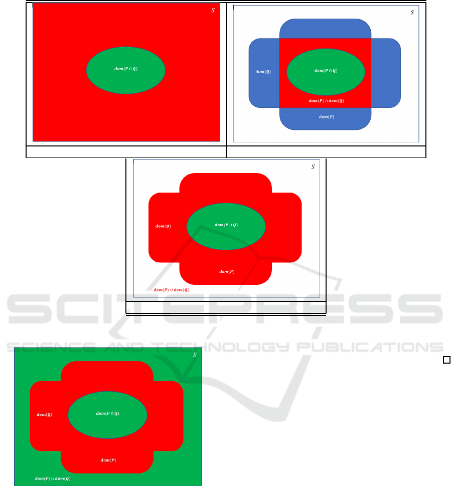
δ
B
(P, Q) δ
S
(P, Q)
δ
L
(P, Q)
Figure 4: Three Definitions of Differentiator Sets.
Figure 5: Fourth Interpretation of Identical Outcome.
respect to the function of program Q (interpreted as a
specification).
Proof. The proof of sufficiency stems readily from
the definition of total correctness (Definition 1) and
the definition of loose differentiator sets.
Proof of Necessity. From δ
L
(P, Q) =
/
0 we infer
dom(P)∪ dom(Q) ⊆ dom(P∩ Q). From which we in-
fer, a fortiori: dom(P) ⊆ dom(P ∩ Q). The reverse
incluse is a tautology. From Definition 1 we infer that
P is totally correct with respect to the function of Q.
In Propositions 2 and 3, the roles of P and Q can
be permuted: each is (partially/ totally) correct with
respect to the function of the other; in the context of
mutation testing, we use these propositions asymmet-
rically,
4 MUTANT SUBSUMPTION
In (Kurtz et al., 2014; Kurtz et al., 2015), Kurtz et al
define the concept of true subsumption as follows:
Definition 4. Given a program P on S and two mu-
tants M and M
′
, we say that M subsumes M
′
with
respect to P if and only if:
P1 There exists an initial state s for which P and M
produce different outcomes.
P2 For all s in S such that P and M produce different
outcomes, so do P and M
′
.
Since this definition makes no mention of P, M
or M
′
failing to converge, we assume that P, M and
Generalized Mutant Subsumption
51
M
′
are considered to converge for all initial states.
The following Proposition formulates subsumption
by means of basic differentiator sets.
Proposition 4. Given a program P on space S and
two mutants M and M
′
of P, M subsumes M
′
if and
only if:
/
0 ⊂ δ
B
(P, M) ⊆ δ
B
(P, M
′
).
Proof. We consider the first condition
/
0 ⊂ δ
B
(P, M)
⇔ {definition of δ
B
(P, M)}
∃s : s ∈
dom(P∩ Q)
⇔ {interpreting the complement}
∃s : ¬(s ∈ dom(P∩ Q))
⇔ {interpreting dom(P∩ Q)}
∃s : ¬(P(s) = Q(s)))
⇔ {definition 4}
Condition P1.
As for the second conditions,
δ
B
(P, M) ⊆ δ
B
(P, M
′
)
⇔ {definition of δ
B
(, )}
∀s : s ∈
dom(P∩ M) ⇒ s ∈ dom(P∩ M
′
)
⇔ {interpreting the complement}
∀s : ¬(s ∈ dom(P∩ M)) ⇒ ¬(s ∈ dom(P∩ M
′
))
⇔ {interpreting the domain}
∀s : ¬(P(s) = M(s)) ⇒ ¬(P(s) = M
′
(s))
⇔ {definition 4}
Condition P2.
The following Proposition reformulates subsump-
tion by means of relative correctness.
Proposition 5. Given a program P on space S and
two mutants M and M
′
of P, M subsumes M
′
if and
only if M is not equivalent to P and it is more-correct
than M
′
with respect to (the function of) P.
Proof. According to Proposition 1, condition P1 is
equivalent to: P and M are not equivalent.
On the other hand, we have shown above that con-
dition P2 is equivalent to:
δ
B
(P, M) ⊆ δ
B
(P, M
′
)
⇔ {definition of δ
B
(, )}
∀s : s ∈
dom(P∩ M) ⇒ s ∈ dom(P∩ M
′
)
⇔ {Boolean identity}
∀s : s ∈ dom(P∩ M
′
) ⇒ s ∈ dom(P∩ M)
⇔ {set theory}
dom(P∩ M
′
) ⊆ dom(P∩ M)
⇔ {Definition 3}
M ⊒
P
M
′
.
Proposition 4 provides an alternative formula to
define mutant subsumption in the case where we as-
sume that all programs and mutants terminate for all
initial states. This Proposition is formulated in terms
of basic differentiator sets, which are defined when
the program and its mutants are assumed to converge
for all initial states; but in section 3, we have in-
troduced two more definitions of differentiator sets,
which do not assume universal convergence of pro-
grams and mutants, and take a liberal interpretation
of program outcomes and when to consider outcomes
as identical or distinct. The following definitions gen-
eralize the concept of subsumption to the case when
programs and their mutants do not necessarily con-
verge for all initial states.
Definition 5. Strict Subsumption. Given a program
P on space S and two mutants M and M
′
of P, we say
that M strictly subsumes M
′
if and only if:
/
0 ⊂ δ
S
(P, M) ⊆ δ
S
(P, M
′
).
Definition 6. Loose Subsumption. Given a program
P on space S and two mutants M and M
′
of P, we say
that M loosely subsumes M
′
if and only if:
/
0 ⊂ δ
L
(P, M) ⊆ δ
L
(P, M
′
).
In the next section,we will see that the distinction
between the basic definition of subsumption (Defini-
tion 4, (Kurtz et al., 2014; Kurtz et al., 2015)), strict
subsumption, and loose subsumption is not a mere
academic exercise. These definitions yield vastly dif-
ferent subsumption graphs.
5 ILLUSTRATION
We consider the Java benchmark pro-
gram of jTerminal (available online at
http://www.grahamedgecombe.com /projects /jtermi-
nal), an open-source software product routinely used
in mutation testing experiments (Parsai and Demeyer,
2017). We apply the mutant generation tool Lit-
tleDarwin in conjunction with a test generation and
deployment class that includes 35 test cases (Parsai
and Demeyer, 2017); we augmented the benchmark
test suite with two additional tests, intended specifi-
cally to trip the base program jTerminal, by causing
to diverge. We let T designate the test augmented
test suite codified in this test class; all our analysis
of mutant equivalence, mutant redundancy, mutant
survival, etc is based on the outcomes of programs
and mutants on this test suite (and carefully selected
subsets thereof). Execution of LittleDarwin on
jTerminal yields 94 mutants, numbered m1 to m94;
the test of these mutants against the original using
the selected test suite kills 48 mutants; for the sake of
documentation, we list them below:
m1, m2, m7, m8, m9, m10, m11, m12, m13,
ICSOFT 2022 - 17th International Conference on Software Technologies
52

m14, m15, m16, m17, m18, m19, m21, m22,
m23, m24, m25, m26, m27, m28, m44, m45,
m46, m48, m49, m50, m51, m52, m53, m54,
m55, m56, m57, m58, m59, m60, m61, m62,
m63, m83, m88, m89, m90, m92, m93.
The remaining 46 mutants are semantically equiva-
lent to the pre-restriction of jTerminal to T. The first
order of business is to partition these 48 mutants into
equivalence classes modulo semantic equivalence;
we find that these 48 mutants are partitioned into 31
equivalence classes, and we select a member from
each class; we let µ be the set of selected mutants:
µ =
m1, m2, m7, m11, m13, m15, m19, m21, m22,
m23, m24, m25, m27, m28, m44, m45, m46, m48,
m49, m50, m51, m52, m53, m55, m56, m57, m60,
m63, m92, m93
.
We resolve to draw the subsumption graphs of
these mutants according to the three definitions:
• Basic/ True Subsumption:
/
0 ⊂ δ
B
( jTerminal, M) ⊆ δ
B
( jTerminal, M
′
).
• Strict Subsumption:
/
0 ⊂ δ
S
( jTerminal, M) ⊆ δ
S
( jTerminal, M
′
).
• Loose Subsumption:
/
0 ⊂ δ
L
( jTerminal, M) ⊆ δ
L
( jTerminal, M
′
).
To this effect, we must compute the differ-
entiator sets δ
B
( jTerminal, M), δ
S
( jTerminal, M),
δ
L
( jTerminal, M) for all 31 mutants selected above,
with respect to jTerminal. For the sake of illustration,
we show in Table 1 the output file of the base program
jTerminal, as well as that of mutant M22; the number
at the start of each line identifies the input. Using this
table, we can derive the differentiator set of M22 with
respect to jTerminal; this is shown in Table 2, under
all. three interpretations (basic, strict, loose) of dif-
ferentiator sets; these sets can be inferred from the
definitions, by analyzing the output files of the base
program and the mutant. The first observation that we
can make about these output files is that divergence,
far from being an exceptional circumstance, is in fact
a very frequent occurrence; notwithstanding the two
instances of divergence that we have triggered on pur-
pose at lines 9 and 10, mutant M22 fails to converge
for several other inputs, which are part of the original
benchmark test suite.
Note that this experiment is artificial in the sense
that whereas the strict and loose definitions of differ-
entiator sets can be applied to the same combination
of program and test suite, the basic definition can only
be applied when we know, or assume, that the base
program and all the mutants converge for all the ele-
ments of the test suite. In the case of jTerminal and its
mutants, this assumption does not hold, as virtually
all of them fail to converge on at least some elements
of T. We obviate this difficulty by considering that
divergence is itself an execution outcome, but this is
merely a convenient assumption for the sake of the
experiment.
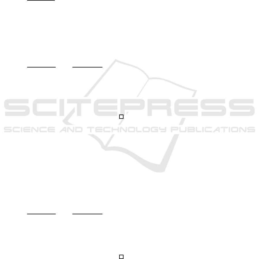
By computing the basic, strict and loose differen-
tiator sets of all the mutants with respect to jTermi-
nal and comparing them for inclusion, we derive the
subsumption relations between the mutants, which we
can represent by graphs; these graphs are given in, re-
spectively, Figures 6, 7 and 8. Nodes in these graphs
represent mutants and arrows represent subsumption
relations: whenever there is an arrow from mutant M
to mutant M
′
, it means that M subsumes M
′
(hence
M
′
can be eliminated from the mutant set without
affecting its effectiveness). When two mutants sub-
sumes each other (for example M27 and M28 in 7),
this means that though these mutants are distinct from
each other (they compute functions functions), they
have the same differentiator set with respect to jTer-
minal.
From these graphs, we derive minimal mutant sets
by selecting the maximal nodes in the subsumption
ordering. Once we have the minimal mutant sets, we
derive minimal test suites that kill all the mutants in
these sets. We verify, in each case, that the test suites
that kills all the mutants of the minimal mutant sets
actually kill all the 48 non-equivalent mutants derived
in our experiment; this comes as no surprise, since
this precisely the rationale for deleting subsumed mu-
tants.
For strict subsumption, for example, we find the
following minimal mutant set:
m22, m23, m27, m28, m44, m45, m48, m50,
m51, m54, m56, m61, m83, m92, m93
.
Using this mutant set, we derive minimal test suites
that kill all these mutants; we find 6 minimal test
suites, of size 7:
Suite 1:
{
t7,t16,t18,t20,t21,t22,t25
}
Suite 2:
{
t7,t16,t18,t20,t21,t22,t26
}
Suite 3:
{
t16,t18,t20,t21,t22,t23,t25
}
Suite 4:
{
t16,t18,t20,t21,t22,t25,t27
}
Suite 5:
{
t16,t18,t20,t21,t22,t23,t26
}
Suite 6:
{
t16,t18,t20,t21,t22,t26,t27
}
By virtue of subsumption, these test suites kill all 31
mutants selected above; by virtue of equivalence, they
necessarily kill all 48 killable mutants of jTerminal.
Using the basic interpretation of subsumption, we
find 96 minimal test suites, all of them of size 12; for
the loose interpretation of subsumption, we find 48
minimal test suites, all of them of size 11. Due to
Generalized Mutant Subsumption
53

Table 1: Outputs of jTerminal and Mutants.
t3, null
t4, c
t5, c
t6, a
t7, null
t8, B
t1, h
t23, com.grahamedgecombe.jterminal.TerminalCell@47089e5f
t24, X
t25, java.awt.Color[r=255,g=0,b=0]
t26, java.awt.Color[r=255,g=255,b=0]
t27, com.grahamedgecombe.jterminal.TerminalCell@4141d797
t28, X
t29, java.awt.Color[r=0,g=0,b=0]
t30, java.awt.Color[r=192,g=192,b=192]
t33, H
t34, i
t35, null
t36, 1
t37, 3
t2, h
t9, java.lang.IndexOutOfBoundsException
t10, java.lang.IndexOutOfBoundsException
t31, 3
t32, 17
t11, A
t12, null
t13, 5
t14, 2
t15, 7
t16, 3
t17, 0
t18, 3
t19, 0
t20, 2
t21, 3
t22, 7
t3, null
t4, java.lang.NullPointerException
t5, java.lang.NullPointerException
t6, java.lang.NullPointerException
t7, com.grahamedgecombe.jterminal.TerminalCell@5f8ed237
t8, java.lang.NullPointerException
t1, h
t23, null
t24, java.lang.NullPointerException
t25, java.lang.NullPointerException
t26, java.lang.NullPointerException
t27, null
t28, java.lang.NullPointerException
t29, java.lang.NullPointerException
t30, java.lang.NullPointerException
t33, java.lang.NullPointerException
t34, java.lang.NullPointerException
t35, java.lang.NullPointerException
t36, 1
t37, 3
t2, h
t9, java.lang.ArrayIndexOutOfBoundsException
t10, java.lang.ArrayIndexOutOfBoundsException
t31, 3
t32, 17
t11, java.lang.ArrayIndexOutOfBoundsException
t12, java.lang.ArrayIndexOutOfBoundsException
t13, 5
t14, 2
t15, 7
t16, 3
t17, 0
t18, 3
t19, 0
t20, 2
t21, 3
t22, 7
Output of Base Program, jTerminal Output File, mutant M22
Table 2: Differentiator Sets of Mutant M22.
Mutant δ
B
δ
S
δ
L
M22
{t4, t5, t6, t7, t8, t23, t24, t25, t26, t27,
t28, t29, t30, t33, t34, t35, t11, t12}
{t23, t27}
{t4, t5, t6, t7, t8, t23, t24, t25, t26, t27,
t28, t29, t30, t33, t34, t35, t11, t12}
space limitations, we do not include these test suites.
Suffice it to say that their number and their size are
vastly different from those found under the strict in-
terpretation.
6 CONCLUSION
In this paper, we seek to generalize the concept of mu-
tant subsumption by analyzing what can be consid-
ered as the outcome of a program, when two program
outcomes can be compared, and under what condition
two comparable program outcomes can be considered
as identical or distinct. To this effect, we introduce
the concept of differentiator set, and find that we can
define three versions of differentiator sets, depending
on how we answer the above-cited questions. Specif-
ically, we consider the following definitions:
• Basic Differentiator Set. The basic differentiator
set of two program P and Q (denoted by δ
B
(P, Q))
is defined only if P and Q converge for all initial
states, and it includes all initial states for which P
and Q yield distinct final states.
ICSOFT 2022 - 17th International Conference on Software Technologies
54
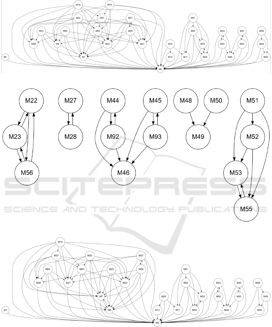
Figure 6: Basic Subsumption Graph, jTerminal Mutants.
Figure 7: Strict Subsumption Graph, jTerminal Mutants.
Figure 8: Loose Subsumption Graph, jTerminal Mutants.
• Strict Differentiator Set. The strict differentiator
set of two programs P and Q (denoted by δ
S
(P, Q))
can be defined regardless of whether P and Q con-
verge for all initial states; it contains all initial
states for which P and Q converge and produce
distinct final states.
• Loose Differentiator Set. The loose differentia-
tor set of two programs P and Q (denoted by
δ
L
(P, Q)) can be defined regardless of whether P
and Q converge for all initial states; it contains all
Generalized Mutant Subsumption
55

initial states for which P and Q converge and pro-
duce distinct final states, as well as all initial states
for which one of them diverges and the other con-
verges, regardless of the final state produced by
the program that converges.
Using these three definitions of differentiator sets, we
get three distinct versions of mutant subsumption:
Mutant M subsumes mutant M
′
with respect to base
program P if and only if:
/
0 ⊂ δ
B
(P, M) ⊆ δ
B
(P, M
′
)
or
/
0 ⊂ δ
S
(P, M) ⊆ δ
S
(P, M
′
)
or
/
0 ⊂ δ
L
(P, M) ⊆ δ
L
(P, M
′
)
depending on our interpretation of program outcomes,
the condition under which we consider that two out-
comes are comparable, and the condition under which
two comparable outcomes are identical.
These three definitions of differentiator sets yield
three distinct definitions of what it means for a test to
kill a mutant; they also yield three distinct subsump-
tion graphs, and three distinct minimal mutant sets.
Indeed, a test t kills a mutant M with respect to base
program P if and only if
t ∈ δ(P, M),
where δ(P, M) can be δ
B
(P, M), δ
S
(P, M), δ
L
(P, M),
depending on the interpretation we adopt. Also, a test
suite T kills a mutant M with respect to base program
P if and only if
T ∩ δ(P, M) 6=
/
0,
where δ(P, M) can be δ
B
(P, M), δ
S
(P, M), δ
L
(P, M),
depending on the interpretation we adopt.
We show by means of a simple example that
different interpretations yield different subsumption
graphs. Among other things, this example highlights
the need to take into consideration the possibility of
divergence, since many of its mutants diverge for
many of the tests included in its benchmark test suite.
ACKNOWLEDGEMENT
The authors are very grateful to the anonymous re-
viewers for their valuable feedback, which has greatly
enhanced the content and presentation of the paper;
they are also genuinely impressed by the thorough-
ness, proficiency and precision of the reviewers’ feed-
back.
This research is partially supported by NSF grant
DGE1565478.
REFERENCES
Brink, C., Kahl, W., and Schmidt, G. (1997). Relational
Methods in Computer Science. Advances in Computer
Science. Springer Verlag, Berlin, Germany.
Dijkstra, E. (1976). A Discipline of Programming. Prentice
Hall.
Gries, D. (1981). The Science of Programming. Springer
Verlag.
Guimaraes, M. A., Fernandes, L., Riberio, M., d’Amorim,
M., and Gheyi, R. (2020). Optimizing mutation test-
ing by discovering dynamic mutant subsumption rela-
tions. In Proceedings, 13th International Conference
on Software Testing, Validation and Verification.
Hoare, C. (1969). An axiomatic basis for computer pro-
gramming. Communications of the ACM, 12(10):576–
583.
Jia, Y. and Harman, M. (2008). Constructing subtle faults
using higher order mutation testing. In Proceed-
ings, Eighth IEEE International Working Conference
on Software Code Analysis and Manipulation, pages
249–258, Beijing, China.
Kurtz, B., Amman, P., Delamaro, M., Offutt, J., and Deng,
L. (2014). Mutant subsumption graphs. In Proceed-
ings, 7th International Conference on Software Test-
ing, Validation and Verification Workshops.
Kurtz, B., Ammann, P., and Offutt, J. (2015). Static analy-
sis of mutant subsumption. In Proceedings, IEEE 8th
International Conference on Software Testing, Verifi-
cation and Validation Workshops.
Li, X., Wang, Y., and Lin, H. (2017). Coverage based dy-
namic mutant subsumption graph. In Proceedings,
International Conference on Mathematics, Modeling
and Simulation Technologies and Applications.
Manna, Z. (1974). A Mathematical Theory of Computation.
McGraw-Hill.
Marsit, I., Ayad, A., Kim, D., Latif, M., Loh, J., Omri,
M. N., and Mili, A. (2021). The ratio of equivalent
mutants: A key to analyzing mutation equivalence.
Journal of Systems and Software.
Mili, A. (2021). Differentiators and detectors. Information
Processing Letters, 169.
Parsai, A. and Demeyer, S. (2017). Dynamic mutant sub-
sumption analysis using littledarwin. In Proceedings,
A-TEST 2017, Paderborn, Germany.
Schmidt, G. (2010). Relational Mathematics. Number 132
in Encyclopedia of Mathematics and its Applications.
Cambridge University Press.
Souza, B. (2020). Identifying mutation subsumption rela-
tions. In Proceedings, IEEE / ACM International Con-
ference on Automated Software Engineering, pages
1388–1390.
Tenorio, M. C., Lopes, R. V. V., Fechina, J., Marinho,
T., and Costa, E. (2019). Subsumption in mutation
testing: An automated model based on genetic algo-
rithm. In Proceedings, 16th International Confer-
ence on Information Technology –New Generations.
Springer Verlag.
Vercammen, S., DeMeyer, S., Borg, M., and Claessens, R.
(2021). Flaky mutants: Another concern for mutation.
In Proceedings, IEEE 2021 International Cconference
on Software Testing, Porto de Galinhas, Brazil.
ICSOFT 2022 - 17th International Conference on Software Technologies
56
