Constructive Model Inference: Model Learning

for Component-based Software Architectures

Bram Hooimeijer

1 a

, Marc Geilen

2 b

, Jan Friso Groote

3,4 c

Dennis Hendriks

5,6 d

and Ramon Schiffelers

4,3 e

Prodrive Technologies, Eindhoven, The Netherlands

Department of Electrical Engineering, Eindhoven University of Technology, Eindhoven, The Netherlands

Department of Mathematics and Computer Science, Eindhoven University of Technology, Eindhoven, The Netherlands

ASML, Veldhoven, The Netherlands

ESI (TNO), Eindhoven, The Netherlands

Department of Software Science, Radboud University, Nijmegen, The Netherlands

Keywords:

Model Learning, Component-based Software, Industrial Application.

Abstract:

Model learning, learning a state machine from software, can be an effective model-based engineering tech-

nique, especially to understand legacy software. However, so far the applicability is limited as models that can

be learned are quite small, often insufﬁcient to represent the software behavior of large industrial systems.

We introduce a novel method, called Constructive Model Inference (CMI). It effectively allows us to learn

the behavior of large parts of the industrial software at ASML, where we developed the method and it is now

being used. The method uses observations in the form of execution logs to infer behavioral models of concur-

rent component-based (cyber-physical) systems, relying on knowledge of their architecture, deployment and

other characteristics, rather than heuristics or counter examples. We provide a trace-theoretical framework,

and prove that if the software satisﬁes certain architectural assumptions, our approach infers the correct re-

sults.

We also present a practical approach to deal with situations where the software deviates from the assump-

tions. In this way we are able to construct accurate and intuitive state machine models. They provide practi-

tioners with valuable insights into the software behavior, and enable all kinds of behavioral analyses.

1 INTRODUCTION

Model-based systems engineering can cope with the

increasing complexity of software (Akdur et al.,

2018). However, for most software, especially legacy

software, no models exist and constructing models

manually is laborious and error-prone.

A solution is to learn the models automatically

from logs of the software. Model inference has been

studied in the ﬁelds of model learning (de la

Higuera, 2010) and process mining (van der Aalst,

2016). Both encompass a vast body of research, and

do not focus speciﬁcally on software systems. Still,

https://orcid.org/0000-0003-0152-4909

https://orcid.org/0000-0002-2629-3249

https://orcid.org/0000-0003-2196-6587

https://orcid.org/0000-0002-9886-7918

https://orcid.org/0000-0002-3297-2969

the techniques have been applied to software compo-

nents in general (Heule and Verwer, 2013; van der

Aalst et al., 2003), and speciﬁcally to legacy compo-

nents (Schuts et al., 2016; Leemans et al., 2018; Bera

et al., 2021).

There are known fundamental limitations to the

capabilities of model inference: Mark Gold has

proven that accurately generalizing a model beyond

observations (logs) is impossible based on observa-

tions alone (Mark Gold, 1967). Accurate learning

from logs requires additional information, such as for

instance counter examples, i.e., program runs that

can never be executed. In practice, often heuristics

are used, based on the input observations (e.g., con-

sidering only the last n events) or the resulting model

(e.g., limiting the number of resulting states).

Alternative to counter examples, active automata

learning queries (parts of) the system (Angluin,

146

Hooimeijer, B., Geilen, M., Groote, J., Hendriks, D. and Schiffelers, R.

Constructive Model Inference: Model Learning for Component-based Software Architectures.

DOI: 10.5220/0011145700003266

In Proceedings of the 17th International Conference on Software Technologies (ICSOFT 2022), pages 146-158

ISBN: 978-989-758-588-3; ISSN: 2184-2833

1987). It guarantees that the inferred models exactly

match the software implementation. But it suffers

from scalability issues (Howar and Steffen, 2018;

Yang et al., 2019; Aslam et al., 2020), limiting the

learned models to a few thousand states at most.

We aim to infer models for large industrial sys-

tems. Our approach therefore learns models from

software execution logs, which are interpreted using

knowledge of the software architecture, its deploy-

ment and other characteristics. It does not rely on

queries or counter examples. It also has no heuristics

that would be hard to conﬁgure correctly, especially

if they do not directly relate to system properties.

We instead inject our knowledge of the system’s

component structure, and the services each compo-

nent provides, which it can implement by invoking

services provided by other components. After a com-

ponent executes a service, it returns a response and is

ready to again provide its services. This knowledge

of the components and their services is essential to

cope with the complexity of the industrial systems

we deal with. It allows us to learn multi-level models

that are small enough for engineers to interpret, while

capturing the complex system behavior of actual

software systems at company ASML, consisting of

dozens of components, with states spaces that are too

large to interpret (i.e., 10

states and beyond). To

the best of our knowledge no similar approach exists.

To demonstrate that our learning approach is ade-

quate, we prove that if a component-based software

architecture satisﬁes our assumptions, our learning

approach returns the correct result, both in settings

with synchronous and asynchronous commu-

nication between the concurrent components. While

the actual software largely adheres to our structural

and behavioral assumptions, there are however parts

that do not. We deal with this by analyzing the

learned models, e.g., by searching for deadlocks. Part

of the approach is a systematic method to add addi-

tional knowledge, to exclude from the models any

behavior known to not be exhibited by the system.

Inspection of the learned models by experts led

to the judgment that the models are very adequate,

and provide them the software behavior abstractions

that they currently lack (Yang et al., 2021). Learning

larger models is limited not by the software size, but

by the capability to analyze those models.

This paper is organized as follows. Section 2

presents an overview of the approach. Section 3 re-

calls basic deﬁnitions. The novel Constructive Model

Inference (CMI) approach, our main contribution, is

described and analyzed, for synchronously and asyn-

chronously composed component-based systems, in

Sections 4 and 5, respectively. Section 6 outlines a

method to apply the approach, using a case study at

ASML as example. Section 7 draws conclusions.

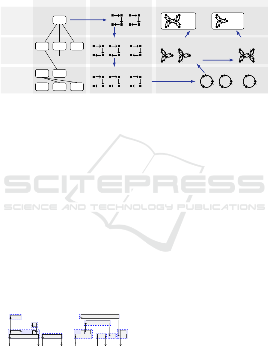
2 CMI OVERVIEW

We present a high-level outline of the method before

discussing the detailed steps in the following sec-

tions. Figure 1 illustrates the overall approach and

the steps involved. The left column shows the as-

sumed system architecture. A system (S) consists of

a known set of components (C

, C

) that collabo-

rate, communicate and use each other’s services. A

component, in turn, consists of the services it offers

, F

). We refer to different functions in the com-

ponent’s implementation that together implement a

service (F

1,1

, F

1,2

, F

1,3

) as service fragments. They

handle incoming communications, e.g., client re-

quests and server responses. We use this architecture

to decompose observations, downwards in the mid-

dle column, and compose models, upwards in the

right column, to reconstruct the system behavior.

The inference method requires observing system

executions (Preparation). The resulting runtime ob-

servations in the form of execution logs, consisting of

events, are the input to our method. Using knowledge

of the system architecture, the observations are ﬁrst

(Step 1) decomposed into observations pertaining to

individual components. Assuming that the beginning

and the end of each service fragment can be identi-

ﬁed, we decompose observations further into

observations of individual service fragments (Step 2).

Then, we infer ﬁnite state automata models of

service fragments from their observations (Step 3),

assuming that offered services may be repeatedly re-

quested, and executed from start to end. The service

fragment models are combined to form component

models (Step 4), where each component repeatedly

executes its services, non-preemptively, one at a

time. These component models are put in parallel to

form the behavior of the system (Step 6).

The learned system model may exhibit behavior

that the real system does not, e.g., due to missing de-

pendencies between service fragments. The method

provides for optional reﬁnement (Step 5), whereby

behavioral constraints derived from the software ar-

chitecture and expert knowledge can be added to the

component models, in a generic and structured way.

Injecting such behavior allows turning stateless ser-

vices into stateful ones, removing non-system

behavior from the models.

The composition in Step 6 can be performed in

various ways, depending on assumptions about the

way the system is composed of components, i.e., ei-

Constructive Model Inference: Model Learning for Component-based Software Architectures

147

System

level

Component

level

Service

(fragment)

level

Architecture

Observations

Behavioral models

... ...

1.1

1.2

1.3

System observations

S S

...

Component observations

... ...

Service fragment observations

1.1

... ...

Service fragment models

1.1

1.2

... ...

Component models (stateless

across service fragments)

...

Component models

(stateful)

...

System model

∥ B

∥ ∥

...

Preparation: Observe

system execution

Step 1: System

decomposition

Step 2: Component

decomposition

Step 3: Service fragment

model inference

Step 4: Service

fragment generalization

Step 5: Stateful

behavior injection

Step 6: Component

composition

Figure 1: Constructive Model Inference (CMI): Overview and its six steps, positioned along abstraction levels (rows) and

conceptual views (columns).

ther synchronously or asynchronously, with varying

buffering and scheduling policies. In the ﬁgure, this

is visualized as the composition of component

models with explicit buffer models (B

, B

Running Example. Figure 2 shows two examples of

observations of the behavior of a component-based

system on a horizontal time axis. The system con-

sists of three components, C

, C

and C

, shown on

the vertical axis. In Figure 2a, component C

receives an incoming request req

from the environ-

ment, and in response executes its service fragment

(function) f , illustrated by the horizontal bar, ulti-

mately leading to a reply rep

. During the execution

of function f , component C

executes function g and

component C

handles it. This involves a remote pro-

cedure call (arrow in the ﬁgure), with request req

being sent to component C

, and after C

has exe-

cuted function g, its reply rep

being received by C

similarly calls h on component C

. After C

be-

comes idle again, a second request req

is received,

and handled in service fragment z, leading to a reply

rep

, this time without involving other components.

In the ﬁgure, the stacked bars for each component

represent call stacks of nested function calls. The

bottom bars represent service fragment function exe-

cutions. Complete call stacks are visualized in the

ﬁgure by enclosing them in blue dashed rectangles.

g h

req

rep

req

rep

req

rep

req

rep

(a)

g h

z hr gr

f r

req

rep

req

rep

req

rep

req

rep

(b)

Figure 2: Observations showing client request req

be-

ing handled by component C

through calls g and h to its

servers, (a) synchronously and (b) asynchronously.

From the start of a service fragment’s call stack, until

its end where it is idle again, this represents a single

observation of its behavior.

Figure 2b shows a different observation of the

system, where request req

is handled asyn-

chronously. Again, services from components C

and

are requested, but now the system does not wait

for their replies. Instead, it completes service frag-

ment f and proceeds to handle request req

. When the

responses from the other components come in (rep

and rep

), it handles these in separate service frag-

ments (hr and gr). Having received both responses, it

sends reply rep

as part of the last service fragment.

Here service fragments f, hr and gr together

implement a service of C

, offered via req

Such system behaviors can be observed in the

form of an execution log, sequences of events in the

order in which they occur in the system. Each start

and end of a function execution (bars in Figure 2) has

an associated event. We identify an event by its exe-

cuting component, the related function, and whether

it represents the start (↑) or the completion (↓) of its

execution. E.g., event f

↑

, abbreviated to f

↑

, denotes

the start of function f on component C

. Where ap-

propriate, we identify service fragments by their start

events, e.g., f

↑

, z

↑

, hr

↑

, gr

↑

, h

↑

and g

↑

for Figure 2.

Our running example has two observations. The

ﬁrst one is the behavior from Figure 2b, i.e., w

= ⟨ f

↑

, g

↑

, g

↓

, h

↑

, h

↑

, h

↓

, f

↓

, z

↑

, z

↓

, h

↓

, hr

↑

, hr

↓

, g

↓

, gr

↑

f r

↑

, f r

↓

, gr

↓

⟩. The second one is a variation of w

where the calls to g and h are reversed, and z handled

last, i.e., w

= ⟨ f

↑

, h

↑

, h

↑

, h

↓

, g

↑

, g

↑

, g

↓

, f

↓

, h

↓

, hr

↑

↓

, g

↓

, gr

↑

, f r

↑

, f r

↓

, gr

↓

, z

↑

, z

↓

⟩. The ﬁgure for w

is omitted for brevity.

ICSOFT 2022 - 17th International Conference on Software Technologies

148

3 PRELIMINARY DEFINITIONS

This section introduces basic deﬁnitions that we build

upon to place our CMI method in a framework based

on ﬁnite state automata and regular languages.

3.1 Finite State Automata

Let Σ be a ﬁnite set of symbols, called an alphabet. A

word (or string) w over Σ is a ﬁnite concatenation of

symbols from Σ. The Kleene star closure of Σ, Σ

∗

, is

the set of all ﬁnite words over Σ, including the empty

word denoted as ε. The Kleene plus closure of Σ is

deﬁned as Σ

= Σ

∗

\ {ε}.

Given a word w, we denote its length as |w|, and

its i

symbol as w

. If words u and v are such that

uv = w, then u is a preﬁx of w and v a sufﬁx of w.

We represent inferred models using DFAs:

Deﬁnition 3.1 (DFA) A deterministic ﬁnite automa-

ton (DFA) A is a 5-tuple A = (Q,Σ, δ,q

,F), with Q a

ﬁnite set of states, Σ a ﬁnite alphabet, δ : Q × Σ → Q

the partial transition function, q

∈ Q the initial state

and F ⊆ Q a set of accepting states.

The transition function is extended to words such

that δ : Q × Σ

∗

→ Q, by inductively deﬁning δ(q,ε) =

q and δ(q, wa) = δ(δ(q,w), a), for w ∈ Σ

∗

, a ∈ Σ. DFA

A = (Q,Σ, δ,q

,F) accepts word w iff state δ(q

,w) ∈

F. If w is not accepted by A, it is rejected. Set L (A) =

{w ∈ Σ

∗

| A accepts w} is the language of A.

A DFA is minimal iff every two states p, q ∈ Q

(p ̸= q) can be distinguished, i.e. there is a w ∈ Σ

∗

such that δ(p,w) ∈ F and δ(q,w) /∈ F, or vice versa.

Given a set of words W ⊆ Σ

∗

, a Preﬁx Tree Au-

tomaton PTA(W ) is a tree-structured acyclic DFA

with L(PTA(W )) = W , where common preﬁxes of W

share their states and transitions.

Given two languages K, L over the same alphabet,

concatenation language KL is {uv | u ∈ K,v ∈ L}. The

repetition of a language L is recursively deﬁned to be

= {ε}, L

i+1

= L

L. Similarly, the repetition of a

word w is w

= ε, w

i+1

= w

w. The Kleene star and

plus closures of L are deﬁned as L

∗

∞

n=0

and

∞

n=1

, respectively.

Given two DFAs A

, A

we deﬁne operations on

DFAs with notations that reﬂect the effect on their re-

sulting languages, i.e., A

∩ A

, A

∪ A

, and A

\ A

result in DFAs with languages L(A

) ∩ L(A

L(A

) ∪ L(A

), and L(A

) \ L(A

), respectively. In

addition, we deﬁne synchronous composition:

Deﬁnition 3.2 (Synchronous Composition) Given

two DFAs A

= (Q

,Σ

,δ

0,1

), A

= (Q

,Σ

0,2

), their synchronous composition, denoted

∥A

, is the DFA:

A = (Q

× Q

,Σ

∪ Σ

,δ,(q

0,1

0,2

),F

× F

with δ((q

),a) deﬁned as:











(δ

,a),δ

,a)) if δ

,a),δ

,a) are deﬁned,

(δ

,a),q

) if δ

,a) is deﬁned, and a /∈ Σ

,δ

,a)) if δ

,a) is deﬁned, and a /∈ Σ

undeﬁned otherwise.

Two DFAs A

are language equivalent, A

⇔

, iff L (A

) = L (A

). Under language equivalence,

each of the operators ⋄ ∈ {∥, ∪,∩} is both commuta-

tive and associative, i.e. A

⋄ A

⇔

⋄ A

and (A

⋄

) ⋄ A

⇔

⋄ (A

⋄ A

To reason about components of a synchronous

composition, we deﬁne word projection:

Deﬁnition 3.3 (Word Projection) Given a word w

over alphabet Σ, and a target alphabet Σ

′

, we deﬁne

the projection π

′

(w) : Σ

∗

→ Σ

′∗

inductively as:

′

(w) =











ε if w = ε,

′

(v) if w = va with v ∈ Σ

∗

,a ̸∈ Σ

′

(v)a if w = va with v ∈ Σ

∗

,a ∈ Σ

′

This deﬁnition is lifted to sets of words:

′

(L) = {π

′

(w) | w ∈ L}.

With word projection, we deﬁne synchronization

of languages, which is commutative and associative:

Deﬁnition 3.4 (Synchronization) Given languages

⊆ Σ

∗

⊆ Σ

∗

, the synchronization of L

and L

the language L

∥L

over Σ = Σ

∪ Σ

such that

w ∈ (L

∥L

) ⇔ π

(w) ∈ L

∧ π

(w) ∈ L

From the deﬁnitions we derive:

Proposition 3.5 Given DFAs A

, A

, their syn-

chronous composition is homomorphic with the

synchronization of their languages: L(A

∥A

) =

L(A

)∥L(A

Proof. For proofs, see (Hooimeijer, 2020).

Corollary 3.6 Given DFAs A, A

, A

such that A =

∥ A

, over alphabets Σ, Σ

, Σ

, respectively, then

w ∈ L(A) ⇔ π

(w) ∈ L(A

) ∧ π

(w) ∈ L(A

3.2 Formalizing Concurrent Behavior

Automata model behavior. To represent concurrent

behavior, Mazurkiewicz Trace theory is introduced

brieﬂy (Mazurkiewicz, 1995). Intuitively, symbols in

the alphabets of multiple automata synchronize in

the synchronous composition (are dependent), while,

e.g., internal non-communicating symbols and

communications involving different components in-

terleave (are independent), and can thus be reordered

or commuted.

Formally, let dependency D ⊆ Σ

× Σ

be a sym-

metric reﬂexive relation over dependency alphabet

Constructive Model Inference: Model Learning for Component-based Software Architectures

149

. Relation I

= (Σ

× Σ

) \ D is the independency

induced by D. Mazurkiewicz trace equivalence for D

is deﬁned as the least congruence ≡

in the monoid

∗

such that for all a, b ∈ Σ

: (a, b) ∈ I

⇒

ab ≡

ba, i.e., the smallest equivalence relation that,

in addition to the above, is preserved under

concatenation: u

≡

∧ v

≡

⇒ u

≡

Equivalence classes over ≡

are called traces. A

trace [w]

for a word w is the set of words equivalent

to w under D. This deﬁnition is lifted to languages:

[L]

= {[w]

| w ∈ L}. We drop subscript D if it is

clear from the context. Language iteration is ex-

tended to traces by deﬁning concatenation of

[u]

, [v]

∈ [Σ

∗

]

as [u]

[v]

= [uv]

, with [u]

preﬁx of [uv]

and [v]

a sufﬁx of [uv]

Given a set T of traces, linT is the linearization of

T , i.e., the set {w ∈ Σ

∗

| [w]

∈ T }. For any string

language L, if L = lin[L]

then L is consistent with

D, as opposed to when L ⊂ lin[L]

. If the language

L(A) of automaton A is consistent with D, A has trace

language T (A) = [L (A)]

Take e.g. Σ

= {a,b,c} and D = {a,b}

∪ {a,c}

= {(a,a),(a, b),(a, c),(b, a),(b,b),(c,a), (c,c)}. As

b and c can then occur independently, I

{(b,c),(c,b)}. Word abbca is part of trace [abbca]

= {abbca, abcba,acbba}, which conﬁrms that

commuting b and c results in the same trace.

The commutation of symbols is captured by bi-

nary relation ∼

, with u ∼

v iff there are x,y ∈ Σ

∗

and (a, b) ∈ I

such that u = xaby and v = xbay.

Clearly, ≡

is the reﬂexive transitive closure of

∼

, i.e. u ≡

v iff there exists a sequence

,...,w

) such that w

= u, w

= v and w ∼

i+1

for 0 ≤ i < n.

We rely on an additional result from

Mazurkiewicz (Mazurkiewicz, 1995):

Proposition 3.7 Given dependency D and words

u,v ∈ Σ

∗

, we have u ≡

v ⇒ π

(u) ≡

(v) for any

alphabet Σ.

3.3 Asynchronous Compositions

In addition to synchronous composition, we intro-

duce asynchronous composition (Akroun and Sala

un,

2018; Brand and Zaﬁropulo, 1983). This makes use

of explicit buffers to pass messages from a sender to

a receiver. For an asynchronous composition of

DFAs A

,...,A

, we assume component A

1 ≤ i ≤ n, has alphabet Σ

, partitioned in sending-,

receiving- and internal-symbols, Σ

, Σ

and Σ

, re-

spectively. Each message has a unique sender and

receiver, Σ

∩ Σ

0, Σ

∩ Σ

0, i ̸= j. The receiver

is assumed to exist, and to be different from the

sender, a ∈ Σ

⇒ ∃

j̸=i

: a ∈ Σ

. Finally, we assume

internal actions are unique to a component,

∩ Σ

0,i ̸= j. We denote an alphabet under these

assumptions as Σ

!,?,τ

The components communicate via buffers, de-

noted B

, which represent, e.g., a FIFO buffer or a

bag buffer. FIFO buffers are modeled as a list of

symbols over Σ

, with ε the empty buffer, where mes-

sages are added to the tail of the list and consumed

from the head of the list. We deﬁne the asynchronous

composition using FIFO buffers as follows:

Deﬁnition 3.8 Consider n DFAs A

,...,A

, with

= (Q

,Σ

!,?,τ

,δ

0,i

), 1 ≤ i ≤ n. The asyn-

chronous composition A of A

,...,A

using FIFO

buffers B

,...,B

, denoted A = ∥

i=1

∥B

), is given

as the (typically inﬁnite) state machine:

A = (Q,Σ,δ, (q

0,1

,ε,...,q

0,n

,ε),F

× ··· × F

)

with Q = Q

× (Σ

)

∗

× ·· · × Q

× (Σ

)

∗

, Σ =

{a!|a ∈ Σ

} ∪

{a?|a ∈ Σ

} ∪

, and

δ ⊆ Q × Σ × Q such that for q = (q

,...,q

)

and q

′

= (q

′

,...,q

′

) we have:

(send) (q, a!,q

′

) ∈ δ if ∃

i, j

: (i) a ∈ Σ

∩ Σ

, (ii)

,a,q

′

) ∈ δ

, (iii) b

′

= b

a, (iv) ∀

k̸=i

′

, (v) ∀

k̸= j

′

= b

(receive) (q,a?, q

′

) ∈ δ if ∃

: (i) a ∈ Σ

, (ii)

,a,q

′

) ∈ δ

, (iii) b

= ab

′

, (iv)

∀

k̸=i

′

= q

, (v) ∀

k̸=i

′

= b

(internal) (q, a,q

′

) ∈ δ if ∃

: (i) a ∈ Σ

, (ii)

,a,q

′

) ∈ δ

, (iii) ∀

k̸=i

′

= q

, (iv)

∀

′

= b

Bag buffers are deﬁned as a multiset over Σ

. To

use bags instead of FIFOs, we change: ε to

0 for A,

list type to multiset type for Q, send rule clause (iii)

to b

′

= b

∪ {a}, and receive rule clause (iii) to a ∈

∧ b

′

= b

− {a}.

With unbounded buffers, asynchronous composi-

tions can have inﬁnite state spaces. When buffers are

bounded, the buffer models can be represented by a

(ﬁnite) DFA (Muscholl, 2010), and hence the compo-

sition as well. We bound buffer B

to k places,

denoted B

, by adding requirement |b

| < k (such

that |b

′

| ≤ k) to the send rule.

We do not discuss the construction of a DFAs for

, as it follows from the deﬁnition above. Then, the

synchronous composition of such constructed DFAs

∥B

is equivalent to asynchronous composition

∥B

as in Deﬁnition 3.8, if for synchronous com-

position we differentiate a! and a? to prevent

synchronization of communications to and from

buffers, respectively.

The question whether there is a buffer capacity

bound such that every accepted word of the un-

bounded composition is also accepted by the

ICSOFT 2022 - 17th International Conference on Software Technologies

150

bounded composition is called boundedness and is

generally undecidable (Genest et al., 2007). How-

ever, if the asynchronous composition is ‘deadlock

free’, i.e. a ﬁnal state can be reached from every

reachable state (Kuske and Muscholl, 2019), then it

is decidable for a given k whether the asynchronous

composition is bounded to k (Genest et al., 2007).

4 CONSTRUCTIVE MODEL

INFERENCE (SYNCHRONOUS

COMPOSITION)

In this section, we detail our method, considering a

system with a synchronous composition of compo-

nents. We later lift the restriction in Section 5, where

we discuss asynchronous compositions.

Recall the CMI method introduced in Section 2,

and its overview in Figure 1. In the previous sections

we introduced the deﬁnitions and the results with

which we can now detail the CMI method.

We assume system execution observations are

available (Preparation step). They are decomposed

following the system architecture (Steps 1 and 2).

Models are then inferred at the most detailed level,

for service fragments (Step 3). Again following the

architecture, inferred models are composed to obtain

models at various levels of abstraction (Steps 4 – 6).

Formally, in this section, we assume the system

under study is a DFA A = (Q,Σ,δ,q

,F), Σ consists

of observable events, A is synchronously composed

of n component DFAs, A = A

∥...∥A

, and that ob-

servations W ⊆ L (A) are available to infer an

approximation A

′

of A. We use subscripts for compo-

nent and service fragment instances, and prime

symbols for inferred instances.

4.1 Step 1: System Decomposition

Informal Description: We assume a ﬁxed and known

deployment of services on components, such that we

can project the observations onto each component.

Formalization: We assume component alphabets Σ

are known a-priori. W is projected to π

(W ) for each

component, 1 ≤ i ≤ n. Recall that we denote events

in Σ as f

, with f a function, C

a component, and s ∈

{↑,↓} denoting the start or completion of a function

execution, e.g., f

↑

. Hence, alphabet Σ

for component

contains the events with subscript i.

Example: Consider again the running example from

Section 2, with W = {w

}. By projection on, e.g.,

component C

, we obtain for both words the projected

word ⟨g

↑

, g

↓

⟩, i.e., π

(W ) = {⟨g

↑

, g

↓

⟩}.

4.2 Step 2: Component Decomposition

Informal Description: We assume that, 1) compo-

nents are sequential (e.g., corresponding to a single

operating system thread), 2) client requests (and

server responses) can only be handled once the com-

ponent is idle, and prior requests are ﬁnished, i.e.,

service fragments are executed non-preemptively,

and 3) symbols that start or end a service fragment

can be distinguished. These assumptions enable us to

decompose component observations into service

fragment observations.

Formalization: A task or task word captures a possi-

ble execution behavior of a service fragment:

Deﬁnition 4.1 (Task) Let Σ be a partitioned alphabet

s,o,e

= Σ

∪ Σ

, with service fragment execution

start events Σ

, its corresponding end events Σ

, and

other events Σ

. Word w ∈ Σ

∗

is a task on component

iff w = f

↑

v f

↓

with f

↑

∈ Σ

, v ∈ Σ

o∗

, and f

↓

∈ Σ

We also deﬁne task sequence and task set:

Deﬁnition 4.2 (Task Sequence/Set) Given alphabet

s,o,e

, a word w ∈ Σ

∗

is a task sequence iff

w = w

...w

with each w

, 1 ≤ i ≤ n, a task. The set

T (w) = {w

|1 ≤ i ≤ n} is the task set corresponding

to w. Similarly T (W ) =

w∈W

T (w) for W ⊆ Σ

∗

Identifying a service fragment by its start event

f ∈ Σ

, its task set is T

(w) = {v | v ∈ T (w) ∧

= f }. T

(W ) ⊆ T (W ) is similarly deﬁned.

For each component C

, given its component

observations π

(W ), we obtain for each service frag-

ment f ∈ Σ

its task set T

(π

(W )), containing the

various observed alternative executions of f .

Example: We get for service fragments f

↑

, z

↑

, hr

↑

, h

↑

, and g

↑

, their respective task sets: {⟨ f

↑

, g

↑

↓

, h

↑

, h

↓

, f

↓

⟩, ⟨ f

↑

, h

↑

, h

↓

, g

↑

, g

↓

, f

↓

⟩}, {⟨z

↑

, z

↓

⟩},

{⟨hr

↑

, hr

↓

⟩}, {⟨gr

↑

, f r

↑

, f r

↓

, gr

↓

⟩}, {⟨h

↑

, h

↓

⟩}, {⟨g

↑

↓

⟩}.

4.3 Step 3: Service Fragment Model

Inference

Informal Description: We infer a DFA per service

fragment. Assuming services may be requested re-

peatedly, each DFA allows its service fragment to

repeatedly be completely executed from start to end.

Formalization: For service fragment f ∈ Σ

, TDFA

constructs a Task DFA (TDFA) from T

(π

(W )), i.e.,

TDFA

(W,Σ

s,o,e

, f ) = A

′

= (Q,Σ

,δ,q

,{q

}). Its

has language L(A

′

) = T

(π

(W ))

∗

, with repeated

executions of its observed set of tasks. An efﬁcient

way to implement TDFA

is to build

Constructive Model Inference: Model Learning for Component-based Software Architectures

151

↑

↓

↑

↓

↑

↓

↑

↓

↑

↓

↑

↓

↑

↓

↑

↓

↑

f r

↑

f r

↓

Figure 3: Task DFAs for the service fragments of the run-

ning example.

PTA(T

(π

(W ))) with root q

. Then, optionally,

minimize the PTA to reduce any redundancy. Finally,

merge all accepting states into initial state q

, which

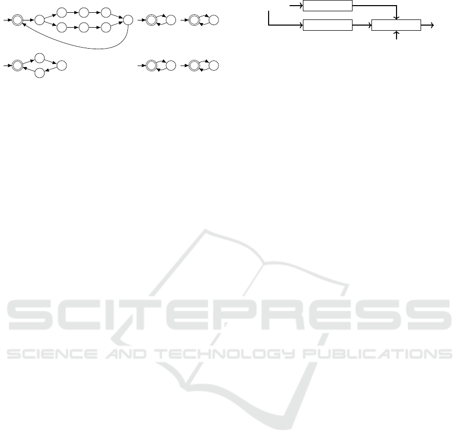
is then the one and only accepting state.

Example: The inferred Task DFAs for the running

example’s service fragments are shown in Figure 3.

4.4 Step 4: Service Fragment

Generalization

Informal Description: We assume components can

repeatedly handle requests of their services. We also

assume (for now, but we revisit this assumption in

Section 4.5) that service executions carry no observ-

able state and are therefore mutually independent.

We infer component models from service fragment

models, generalizing the component behavior to re-

peated non-preemptive executions of the various

service fragments. A component is thus assumed to

be able to execute any number of any of its service

fragments in arbitrary order.

Formalization: For a component C

, its service frag-

ments are Σ

= Σ

∩ Σ

. TDFA

constructs TDFA A

for component C

, i.e., TDFA

(W,Σ

s,o,e

,Σ

) = A

′

. It

does so by merging the initial states of all TDFAs

′

= TDFA

(W,Σ

s,o,e

, f ) for service fragments

f ∈ Σ

. Then L(A

′

) = T (π

(W ))

∗

. A

′

is determinis-

tic, as all outgoing transitions from the initial states

of TDFAs A

′

, i.e., f

↑

, are unique.

Example: The component models for C

and C

are

identical to their service fragment models, for h

↑

and

↑

, respectively, in Figure 3. For C

, the initial states

of its four service fragment models are merged.

4.5 Step 5: Stateful Behavior Injection

Informal Description: In Step 4 we assumed service

fragments to be mutually independent. This is not

always the case in practice. Consider our running ex-

ample (Figure 2b in Section 2). Service fragment f

handles the responses for asynchronous calls g and h

Observations

Steps 1-4

Mining Composition

Model

Manually speciﬁed automata

Figure 4: Generic approach to inject speciﬁc domain knowl-

edge in Step 5.

in service fragments gr and hr, respectively. There-

fore, handling gr always comes after call g in f . This

is ensured by the interaction with C

, but it is not

captured in the model for C

Optional Step 5 allows to inject stateful behavior

to obtain stateful models that exclude behavior that

cannot occur in the real system. As many varieties of

component-based systems exist, our structured ap-

proach allows to improve the inferred models based

on injection of domain knowledge. This allows cus-

tomization to ﬁt a certain architecture or target

system, and is not speciﬁc to our case of Section 6.

E.g., it allows to capture the general property that ‘a

response must follow a request’ (gr after g).

Figure 4 visualizes the approach. We compose

TDFAs inferred in Steps 1 – 4 with additional, typi-

cally small, automata, which specify explicitly which

behavior we add, constrain or remove. Multiple dif-

ferent composition operators are supported: union,

intersection, synchronous composition and (symmet-

rical) difference (see Section 3). The injected

automata are manually speciﬁed, or obtained by a

miner (Beschastnikh et al., 2013), an automated

procedure on the observations.

Additional properties that should be added often

apply in identical patterns across the whole system.

To allow modeling them only once, DFAs with pa-

rameters are used, e.g., for the pattern of a request

and reply. The parameterized DFA (template) is in-

stantiated for speciﬁc symbols, e.g. user-provided

request/reply pairs, to obtain the DFAs to inject.

Formalization: We deﬁne substitution:

Deﬁnition 4.3 (Substitution) Given a parameterized

DFA A = (Q,Σ, δ,q

,F), and symbols p ∈ Σ, a /∈ Σ,

the substitution of a for p in A, denoted A[p := a],

is deﬁned as A[p := a] = (Q,(Σ \ {p}) ∪ {a},δ[p :=

a],q

,F), with δ[p := a](q,c) = δ(q, p) if c = a, and

δ(q,c) otherwise.

In general the order of substitutions matters. We

apply them in the given order, and only replace pa-

rameter symbols by concrete symbols, assuming

both sets are disjoint.

Example 1 (Request before Reply): For asynchronous

calls, a reply must follow a request, e.g., gr after g.

We model this property as DFA P

in Figure 5a. Pa-

rameter Req represents a request, Reply a reply. To

ICSOFT 2022 - 17th International Conference on Software Technologies

152

Req

(a)

1 2

cReq

cReply

sReq

sReply

(b)

Figure 5: Parameterized property automata: (a) request be-

fore reply (P

), (b) server replies before client reply (P

enforce the property, we compose the inferred

TDFAs A

′

with P

, for every request and its corre-

sponding reply in the system being considered:

′′

= A

′

∥ (∥

a∈reqs

[Req := a][Reply := R(a)]),

where reqs is the set of requests, and R : Σ

→ Σ

maps requests to their replies. E.g., for our example,

↓

∈ reqs and (g

↓

,gr

↑

) ∈ R. By Corollary 3.6, for any

a ∈ reqs: π

{a,R(a)}

(L(A

′′

)) = {(a.R(a))

| n ∈ N}.

This correctly models the informally given property,

assuming at most one outstanding request for each a.

Example 2 (Server Replies before Client Reply): For

a service execution, often nested requests should have

been replied before ﬁnishing the service. We model

this property as DFA P

in Figure 5b. Upon receiving

a client request cReq, P

goes to state 2. If during this

service, a request sReq is sent to a server, it must be

met with reply sReply to get out of state 3 and allow

the original service to reply to its client (cReply).

The examples show that domain knowledge can

be added explicitly, straightforwardly, and with

parameterized DFAs and miners also scalably.

4.6 Step 6: Component Composition

Informal Description: The last step is to form system

models by composing the obtained stateless and/or

stateful component models (from Steps 4 and 5).

Formalization: So far we have used unique symbols

per component, such as, e.g., f

↑

. Properly capturing

component synchronization requires that we ensure

the correct communications when one components

uses the services of another component. For our

running example (see Figure 2b), we have a commu-

nication (arrow) from g

↑

to g

↑

. To ensure correct

synchronization, we use the same symbol for both of

them. We combine g

↑

and g

↑

to the synchronization

action g

↑,↑

1,3

, representing the start of call g on C

lead-

ing to the immediate start of a handler for g on C

Then synchronous composition can be applied to di-

rectly obtain A

′

= A

′

∥A

′

∥...∥A

′

as per

Deﬁnition 3.2.

Example: We omit the resulting system model

automaton for brevity.

4.7 Analysis of the CMI Method

Steps 1 and 6: These steps together reduce the

problem of inferring system models from system ob-

servations to inferring component models from

component observations. We ﬁrst analyze four as-

pects purely for this reduction, without considering

that, e.g., other steps allow repeated (task) execution.

Hence, for now we consider PTAs, not TDFAs. And

word length of observations is preserved, even after

commutations for Mazurkiewicz trace equivalence.

1) We prove that composition A

′

= A

′

∥...∥A

′

of in-

ferred components A

′

accepts the original system

observations W from which it was inferred, i.e.,

W ⊆ L (A

′

). By deﬁnition, if A

′

= PTA(W ) then

L(A

′

) = W . We have A

′

= PTA(π

(W )) instead, for

each i. Then by Corollary 3.6 this follows directly.

2) We show that composition A

′

generalizes to traces,

using Mazurkiewicz trace theory. That is, it properly

uses concurrency between components to accept all

valid alternative interleavings that were not directly

observed, i.e., learning a PTA per component

generalizes L(A

′

) from W to lin[W ]

Proposition 4.4 If dependency D =

i=1

(Σ

), u,v ∈

∗

, Σ =

i=1

, then u ≡

v ⇔ ∀

: π

(u) = π

(v).

Corollary 4.5 For a synchronous composition A =

∥...∥A

and D =

i=1

(Σ

), L(A) = lin[L (A)]

Per Proposition 4.4 and Corollary 4.5, decompos-

ing the system to components preserves commuta-

tions, and all commutated words are indeed in L(A

′

3) We show A

′

does not over-generalize A. That is,

the inferred model has no behavior that the original

system does not have, i.e., L(A

′

) ⊆ L (A). As A and A

′

both generalize to traces per Corollary 4.5, and given

W ⊆ L (A), this follows directly. Together this leads

to the following theorem:

Theorem 4.6 Consider DFA A = ∥

i=1

, W ⊆ L (A),

DFA A

′

= ∥

i=1

′

with A

′

= PTA(π

(W )), and D =

i=1

(Σ

). Then L (A

′

) = lin[W ]

and L(A

′

) ⊆ L(A).

Generally, it is sufﬁcient to show this per component:

Proposition 4.7 If L(A

′

) ⊆ L(A

) and

L(A

′

) ⊆ L(A

), then L(A

′

∥ A

′

) ⊆ L(A

∥ A

4) A

′

is robust under additional observations, i.e., if

inference uses additional observations, then the

language of the inferred model can only grow:

Theorem 4.8 Consider DFA A

′

= ∥

i=1

′

with

′

= PTA(π

(U)), obtained from observations U ,

and DFA A

′′

, similarly composed and obtained from

observations V , with U ⊆ V . Then L(A

′

) ⊆ L(A

′′

Steps 2 – 4: Steps 2 and 4 together reduce the prob-

lem of inferring component models from component

Constructive Model Inference: Model Learning for Component-based Software Architectures

153

∥

b b

c a

(a)

∥

a a

(b)

Figure 6: (a) TDFAs X

′

∥X

′

= X

′

, (b) TDFAs Y

′

||Y

′

observations to inferring service fragment models

from service fragment observations, which is real-

ized by Step 3. We analyze the four aspects as

before, plus an extra one. Unlike before, we now do

consider repeated (task) executions and TDFAs.

1) We show that our approach produces correct com-

ponent Task DFAs A

′

, and that composition

′

= A

′

∥...∥A

′

then still accepts W :

Proposition 4.9 Consider DFA A with Σ

s,o,e

com-

posed of Task DFAs, A = ∥

i=1

with each a Σ

∩ Σ

, observations W ⊆ L(A), and DFAs A

′

TDFA

(W,Σ

s,o,e

,Σ

). Then L (A

′

) = T (π

(W ))

∗

Proposition 4.9 follows by construction. Then, by

Corollary 3.6, also W ⊆ L (A

′

) still holds.

2) We consider how A

′

generalizes observations. A

composition A

′

of TDFAs A

′

is not generally a Task

DFA. Even if a symbol is only in Σ

for all compo-

nents, transitions for that symbol might not go to the

accepting state (e.g. abac over Figure 6a). Yet, by

Proposition 3.5, we know that any word in the

language of A represents executions of tasks on com-

ponents. Hence, we extend tasks to task traces and

task sequences to task sequence traces:

Deﬁnition 4.10 (Task (Sequence) Trace) Consider a

dependency D =

i=1

and alphabet Σ

s,o,e

. A trace

[t] ∈ [Σ

∗

] is a task sequence trace iff ∀

i=1

(t) is a

task sequence for Σ

s,o,e

. Its task set T([t]), is given

as {[t

] | [t

... t

] = [t] and t

a task for 1 ≤ j ≤ m}.

If additionally, no task sequences [u],[v] ∈ [Σ

] exist

such that [uv] = [t], then [t] is not a concatenation of

multiple task traces, but a single task trace.

Using task traces, we deﬁne how a composition of

concurrently executing components generalizes, i.e.,

what commutations are possible:

Proposition 4.11 Consider a composition A = ∥

i=1

of n Task DFAs, with dependency D =

i=1

. Then

any [t] ∈ T (A) is a task sequence, and furthermore

[t] ∈ T (A) ⇔ T ([t]) ⊆ T (A), and T (A) = T (T (A))

∗

For the TDFAs in Figure 6a, Mazurkiewicz traces

allow us to deﬁne T (X

′

) = T([abacbc])

∗

= {abc,

abacbc}

∗

. Clearly, T (X

′

) allows commutations, as

abc ∈ T (X

′

), while abc /∈ T (abacbc)

∗

Corollary 4.5 earlier showed that A

′

generalizes

to trace equivalence, [W ] ∈ T (A

′

). Proposition 4.11

proves even more generalization: all task traces in W

can be repeated in any order T ([W ])

∗

⊆ T (A

′

However, A

′

generalizes beyond T ([W ])

∗

. For

Figure 6a, L (X

′

) = ab(acb)

∗

c, beyond T (X

′

). Con-

sider also Y

′

and Y

′

in Figure 6b, inferred from

W = {abcacd} for Σ

= {a,d} and Σ

= {a,b, c}.

Here, [w] is a task, as aad cannot be split. Yet

′

= Y

′

∥Y

′

also accepts w

′

= abcabcd and

′′

= acacd, outside T ([W ])

∗

. Y

′

accepts tasks ac

and abc that synchronize equally with Y

′

and can

thus be interchanged. Therefore, characterizing the

full generalization remains an open problem.

3) The inferred component models A

′

do not over-

generalize, i.e., L (A

′

) ⊆ L (A

), per Proposition 4.9

and since π

(W ) ⊆ T (π

(W ))

∗

. Then for A

′

also

still L(A

′

) ⊆ L(A), per Proposition 4.7.

4) Allowing for repeated task executions, A

′

is still

robust under additional observations:

Theorem 4.12 Consider DFA A

′

= ∥

i=1

′

, with A

′

TDFA

(U,Σ

s,o,e

,Σ

) obtained from observations U,

and DFA A

′′

similarly composed and obtained from

observations V , with U ⊆ V . Then L(A

′

) ⊆ L(A

′′

5) Finally, we consider completeness. To infer the

complete behavior of system A, its component task

sets T (L(A

)) should at least be ﬁnite, as we enumer-

ate these tasks in approximations A

′

. If all tasks of A

are observed, the full system behavior is inferred.

5 CONSTRUCTIVE MODEL

INFERENCE

(ASYNCHRONOUS

COMPOSITION)

In Section 4 we considered systems consisting of

synchronously composed components. This section

considers the CMI approach applied to systems with

asynchronously composed components.

We now assume the system is a DFA A, asyn-

chronously composed of components A

, using

buffers B

bounded to capacity b

. Per Section 3.3 we

model this as a synchronous composition with buffer

automata, A = ∥

i=1

∥B

). Then A

has alphabet

!,?,τ

, Σ

= Σ

∪ Σ

, Σ

= {a! | a? ∈ Σ

}, and

= Σ

. We assume system observations W ⊆ L (A)

as before.

To infer A

′

, we ﬁrst infer the components A

′

reusing Steps 1–5 from the synchronous case of Sec-

tion 4. Then, we model DFA buffers B

′b

as in

Section 3.3, according to the buffer type (FIFO or

bag) and capacity bound b

. A capacity lower bound

ICSOFT 2022 - 17th International Conference on Software Technologies

154

req

rep

req

rep

req

Figure 7: Example of limited commutations for FIFO

buffers.

i,w

for each buffer B

is inferred from W, by consid-

ering the maximally occupied buffer space along

each observed word w ∈ W . That is b

i,w

max

1≤i≤|w|

(|π

...w

)| − |π

...w

)|).

Then, the overall lower bound b

for B

is inferred, as

= max

w∈W

i,w

. Finally, A

′

is given as synchronous

composition A

′

= ∥

i=1

′

∥B

′b

Just as for the synchronous case, we prove for

this asynchronous version of Step 6, that A

′

accepts

W , does not over-generalize, and is robust under

additional observations:

Proposition 5.1 Consider DFA A = ∥

i=1

∥B

)

with B

a FIFO (or bag) buffer, W ⊆ L (A), DFA A

′

∥

i=1

′

∥B

′b

) with A

′

= TDFA

(W,Σ

s,o,e

,Σ

), and

′b

a FIFO (or bag) buffer with b

= max

w∈W

i,w

Then W ⊆ L (A

′

) ⊆ L(A). For DFA A

′′

, similarly

composed and obtained from observations V , with

W ⊆ V , then holds L(A

′

) ⊆ L(A

′′

With this approach we need to know a-priori the

kind of buffers used in our system. To understand

whether our choices were correct we experimented

with various buffer types. For instance, using a sin-

gle FIFO buffer between each pair of components

can lead to an issue shown in Figure 7. If req

sent before rep

, the FIFO order enforces reception

of req

before rep

, while the TDFA for C

has to

handle rep

before starting a new service with req

leading to a deadlock. In order to resolve this

problem, and other mismatches with ASML’s mid-

dleware, we use a FIFO buffer per client that a

component communicates with, and a bag per server.

6 CMI IN PRACTICE

We demonstrate our CMI approach by applying it to

a case study at ASML. ASML designs and builds

machines for lithography, which is an essential step

in the manufacturing of computer chips.

Figure 8: Per component, the number of states in its compo-

nent model after Step 4, compared to the number of events

in its observations.

6.1 System Characteristics

Our CMI approach requires as input system observa-

tions. The middleware in ASML’s systems has been

instrumented to extract Timed Message Sequence

Charts (TMSCs) from executions. A TMSC (Jonk

et al., 2020) is a formal model for system observa-

tions, akin to what we described in Section 2. The

TMSC formalism implies that the system can be

viewed as a composition of sequential components

bearing nested, fully observed, non-preemptive

function executions. We can therefore obtain obser-

vations W , component alphabets Σ

, and partitioned

alphabet Σ

s,o,e

, from TMSCs, to serve as inputs to

our method.

For this case study, we infer a model of the expo-

sure subsystem, which exposes each ﬁeld (die) on a

wafer. By executing a system acceptance test, and

observing its behavior during the exposure of a sin-

gle wafer, which spans about 11 seconds, a TMSC is

obtained that consists of around 100,000 events for

33 components.

6.2 Model Inference Steps 1 – 4

We apply Steps 1 – 4 for our case study. Figure 8

shows the sizes of the resulting component models in

terms of the number of events in the observations and

the number of states of the inferred models. For most

components the inferred model is two orders of mag-

nitude more compact than its observations, showing

repetitive service fragment executions in these

components.

Component 1 orchestrates the wafer exposure. Its

model has the same size as its observation, as it spans

a single task with over 5,000 events. For components

26 – 33, the small reduction is due to their limited ob-

servations.

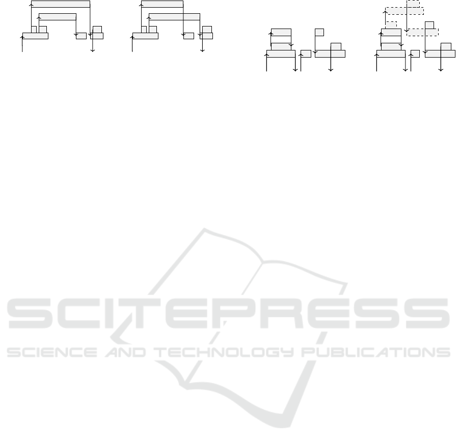
6.3 Model Inference Step 5

We analyze the inferred models, assessing whether

their behavior is in accordance with what we expect

Constructive Model Inference: Model Learning for Component-based Software Architectures

155

h g

gr hr

f r

req

rep

req

rep

req

rep

(a)

h g

hr gr

f r

req

rep

req

rep

req

rep

(b)

Figure 9: Component C

requires both rep

and rep

to re-

ply to its client. (a) gr before hr, with fr in hr, and (b) hr

before gr, with fr in gr.

from the actual software and if not, what knowledge

must be added (according to Step 5).

Although the system matches an asynchronous

composition of components as discussed in Sec-

tion 5, we ﬁrst apply our CMI approach for

synchronous systems (Step 6 from Section 4). A syn-

chronous composition has more limited behavior

compared to an asynchronous composition, and

hence a smaller state space. The resulting model can

therefore be analyzed for issues more easily, while

many such issues apply to both the synchronous and

the asynchronous compositions.

We observe that component model 1, A

′

, has over

5,000 states, in a single task w. To reduce the model

size, we analyze w for repetitions and reduce it

(Nakamura et al., 2013). We look for short

x,y, z ∈ Σ

∗

such that w = xy

z for some n. Then, we

create reduced model A

′′

, with L(A

′′

) = (xyz)

∗

. This

reduces the model size by |y| ∗ (n − 1) states to about

600 states for Component 1, without limiting its

synchronization with the other components.

As a second reduction, we remove DFA transi-

tions that do not communicate and originate from a

state which has a single outgoing transition, i.e. does

not allow for a choice in the process. This is akin to

process algebra axiom a.τ.b = a.b, where τ is a non-

synchronizing action (Milner, 1989). Examples in

Figure 9 are g

↓

and f

↓

. This further reduces A

′′

from

about 600 to about 300 states. Other components are

reduced as well.

With these two reductions, exploring the resulting

state space becomes feasible, being approximately

states. We look for deadlocks: states without

outgoing transitions. As our learned model repre-

sents actual software, we expect no deadlocks. If a

deadlock arises, it is due to a synchronizing symbol,

the counterpart of which cannot be reached.

A ﬁrst issue is illustrated in Figure 9. Component

requests services g and h concurrently. Both are

called asynchronously and can return in either order,

with only the last reply leading to rep

. The inferred

‘stateless’ model does not capture the dependency

between replies rep

, rep

and rep

. When in the

learned model both, or neither, incoming replies are

followed by rep

, the system deadlocks, as the call-

k e

∗

g e

req

rep

req

rep

req

rep

(a)

k e

∗

req

rep

req

rep

req

rep

trg

(b)

Figure 10: Component C

communicates with components

outside the observations, causing missing dependencies.

ing environment expects exactly one reply. This is

solved by enforcing nested services to be ﬁnished be-

fore ﬁnishing f , as in Example 2 from Step 5 of

Section 4.5.

A second issue is illustrated in Figure 10, where

component C

deals with server S

∗

. However, we do

not observe S

∗

directly, but merely through the mes-

sages obtained at C

. The server S

∗

, which S

∗

uses,

is not observed at all. The observation is shown in

Figure 10a, and a possible perspective of the actual

system is shown in Figure 10b.

Since we do not observe S

∗

and S

∗

, the model

misses the dependency between functions g and e

Now, e

has no incoming message and it is able to

start ‘spontaneously’. The actual system relies on the

dependency, and as it is missing in the learned be-

haviour, it has deadlocks. Knowing the missing

dependency from domain knowledge, we inject it

through Step 5 as a one-place buffer similar to

Figure 5a, extended to multiple places as needed.

After resolving these issues, we analyze choices.

From other observations we know that g is optional

when performing f in component C

of Figure 9a.

The inferred model thus contains tasks which have a

common preﬁx, i.e. ⟨ f

↑

↓

, f

↓

⟩ (g is skipped),

and ⟨ f

↑

↓

↑

↓

, f

↓

⟩ (g is called). After h

↓

choice arises, to either call g by g

↑

or ﬁnish f by f

↓

Such choices can enlarge the state space, and may

not apply in all situations. We therefore asked do-

main experts on which information in the software

such a choice could depend. Together, we concluded

that g is only skipped once, and this relates to the

repetitions we observed for C

, as g is skipped for

one particular such iteration. We ensured the correct

choice is made, by constraining the two options to

their corresponding iterations on C

, thus removing

some non-system behavior from the inferred model.

6.4 Model Inference Step 6

To the result of Step 5, we apply asynchronous com-

position (Step 6, Section 5). Using FIFO and bag

buffers as described in that section, service fragments

ICSOFT 2022 - 17th International Conference on Software Technologies

156

are allowed to commute due to execution and

communication time variations.

For our case study, all inferred buffer capacities

are either one or two, except component C

, which has

buffers with capacities up to 24. The low number of

buffer places is due to the extensive synchronization

on replies. C

, the log component, only receives ‘ﬁre-

and-forget’-type logging notiﬁcations without replies.

We veriﬁed that the resulting, improved, asyn-

chronously composed model indeed accepts its input

TMSC, i.e., the inferred model accepts the input ob-

servation from which it was inferred. This gives trust

that the practically inferred model is in line with that

observation. The inferred models were conﬁrmed by

domain experts as remarkably accurate, allowing

them to discuss and analyze their system’s behavior.

This in stark contrast to models that were previously

inferred using process mining and heuristics-based

model learning, where they questioned the accuracy

of the models instead.

7 CONCLUSIONS AND FUTURE

WORK

We introduced our novel method, Constructive

Model Inference (CMI), which uses execution logs

as input. Relying on knowledge of the system archi-

tecture, it allows learning the behavior of large

concurrent component-based systems. The trace-

theoretical framework provides a solid foundation.

ASML considers the state machine models resulting

from our method accurate, and the service fragment

models in particular also highly intuitive. They see

many potential applications, and are already using

the inferred models to gain insight into their software

behavior, as well as for change impact analysis.

Future work includes among others extending the

CMI method to inferring Extended Finite Automata

and Timed Automata, further industrial application

of the approach, and automatically deriving interface

models from component models.

ACKNOWLEDGEMENTS

This research is partly carried out as part of the

Transposition project under the responsibility of ESI

(TNO) in co-operation with ASML. The research ac-

tivities are partly supported by the Netherlands

Ministry of Economic Affairs and TKI-HTSM.

REFERENCES

Akdur, D., Garousi, V., and Demir

ors, O. (2018). A survey

on modeling and model-driven engineering practices

in the embedded software industry. Journal of Systems

Architecture, 91(October):62–82.

Akroun, L. and Sala

un, G. (2018). Automated veriﬁcation

of automata communicating via FIFO and bag buffers.

Formal Methods in System Design, 52(3):260–276.

Angluin, D. (1987). Learning regular sets from queries

and counterexamples. Information and Computation,

75(2):87–106.

Aslam, K., Cleophas, L., Schiffelers, R., and van den Brand,

M. (2020). Interface protocol inference to aid under-

standing legacy software components. Software and

Systems Modeling, 19(6):1519–1540.

Bera, D., Schuts, M., Hooman, J., and Kurtev, I. (2021).

Reverse engineering models of software interfaces.

Computer Science and Information Systems.

Beschastnikh, I., Brun, Y., Abrahamson, J., Ernst, M. D.,

and Krishnamurthy, A. (2013). Unifying FSM-

inference algorithms through declarative speciﬁca-

tion. Proceedings - International Conference on Soft-

ware Engineering, pages 252–261.

Brand, D. and Zaﬁropulo, P. (1983). On Communicating

Finite-State Machines. Journal of the ACM (JACM),

30(2):323–342.

de la Higuera, C. (2010). Grammatical Inference. Cam-

bridge University Press, New York, 1st edition.

Genest, B., Kuske, D., and Muscholl, A. (2007). On com-

municating automata with bounded channels. Funda-

menta Informaticae, 80(1-3):147–167.

Heule, M. J. and Verwer, S. (2013). Software model syn-

thesis using satisﬁability solvers. Empirical Software

Engineering, 18(4):825–856.

Hooimeijer, B. (2020). Model Inference for Legacy Soft-

ware in Component-Based Architectures. Master’s

thesis, Eindhoven University of Technology.

Howar, F. and Steffen, B. (2018). Active automata learning

in practice. In Bennaceur, A., H

ahnle, R., and Meinke,

K., editors, Machine Learning for Dynamic Soft-

ware Analysis: Potentials and Limits: International

Dagstuhl Seminar 16172, Dagstuhl Castle, Germany,

April 24-27, 2016, Revised Papers, pages 123–148,

Cham. Springer International Publishing.

Jonk, R., Voeten, J., Geilen, M., Basten, T., and Schiffelers,

R. (2020). SMT-based veriﬁcation of temporal proper-

ties for component-based software systems. Technical

Report ES Reports, Eindhoven University of Technol-

ogy, Department of Electrical Engineering, Electronic

Systems Group, Eindhoven.

Kuske, D. and Muscholl, A. (2019). Communicat-

ing Automata. Submitted for peer review (Jour-

nal unknown) Retrieved from http://eiche.theoinf.tu-

ilmenau.de/kuske/Submitted/cfm-ﬁnal.pdf.

Leemans, M., van der Aalst, W. M., van den Brand, M. G.,

Schiffelers, R. R., and Lensink, L. (2018). Soft-

ware Process Analysis Methodology – A Methodol-

ogy based on Lessons Learned in Embracing Legacy

Software. In 2018 IEEE International Conference on

Constructive Model Inference: Model Learning for Component-based Software Architectures

157

Software Maintenance and Evolution (ICSME), pages

665–674. IEEE.

Mark Gold, E. (1967). Language identiﬁcation in the limit.

Information and Control, 10(5):447–474.

Mazurkiewicz, A. (1995). Introduction to Trace Theory. In

Diekert, V. and Rozenberg, G., editors, The Book of

Traces, chapter 1, pages 3–41. World Scientiﬁc, Sin-

gapore.

Milner, R. (1989). Communication and Concurrency.

Prentice-Hall, Inc., River, NJ, United States.

Muscholl, A. (2010). Analysis of communicating automata.

In LATA 2010: Language and Automata Theory and

Applications, pages 50–57.

Nakamura, A., Saito, T., Takigawa, I., and Kudo, M. (2013).

Fast algorithms for ﬁnding a minimum repetition rep-

resentation of strings and trees. Discrete Applied

Mathematics, 161(10-11):1556–1575.

Schuts, M., Hooman, J., and Vaandrager, F. (2016). Refac-

toring of Legacy Software using Model Learning and

Equivalence Checking: an Industrial Experience Re-

port. In Integrated Formal Methods: 12th Interna-

tional Conference, pages 311–325.

van der Aalst, W. (2016). Process Mining. Springer-Verlag

Berlin Heidelberg, Berlin Heidelberg, 2nd edition.

van der Aalst, W. M., van Dongen, B. F., Herbst, J.,

Maruster, L., Schimm, G., and Weijters, A. J. (2003).

Workﬂow mining: A survey of issues and approaches.

Data and Knowledge Engineering, 47(2):237–267.

Yang, N., Aslam, K., Schiffelers, R., Lensink, L., Hendriks,

D., Cleophas, L., and Serebrenik, A. (2019). Improv-

ing Model Inference in Industry by Combining Active

and Passive Learning. SANER 2019 - Proceedings of

the 2019 IEEE 26th International Conference on Soft-

ware Analysis, Evolution, and Reengineering, pages

253–263.

Yang, N., Schiffelers, R., and Lukkien, J. (2021). An in-

terview study of how developers use execution logs in

embedded software engineering. In 2021 IEEE/ACM

43rd International Conference on Software Engineer-

ing: Software Engineering in Practice (ICSE-SEIP),

pages 61–70.

ICSOFT 2022 - 17th International Conference on Software Technologies

158