Preprocessing of Terrain Data in the Cloud using a Workﬂow

Management System

Marvin Kaster

1,2 a

and Hendrik M. W

urz

1,2 b

Fraunhofer Institute for Computer Graphics Research IGD, Fraunhoferstraße 5, Darmstadt, Germany

Technical University of Darmstadt, Karolinenplatz 5, Darmstadt, Germany

Keywords:

Cloud Computing, Geospatial Data, Workﬂow Management, Computational Models for Big Data.

Abstract:

The preparation of terrain data for web visualization is time-consuming. We model the problem as a scientiﬁc

workﬂow that can be executed by a workﬂow management system (WMS) in a cloud-based environment. Such

a workﬂow management system provides easy access to the almost unlimited resources of cloud infrastructure

and still allows a lot of freedom in the implementation of tasks. We take advantage of this and optimize the

computation of individual tiles in the created level of detail (LOD) structure, as well as the scheduling of

tasks in the scientiﬁc workﬂow. This enables us to utilize allocated resources very efﬁciently and improve

computation time. In the evaluation, we analyze the impact of different storage endpoints, the number of

threads, and the number of tasks on the run time. We show that our approach scales well and outperforms our

previous work based on the framework GeoTrellis considerably (Kr

amer et al., 2020).

1 INTRODUCTION

In recent years, workﬂow management systems

(WMS) have gained popularity. In the past, tasks

were simple enough to be solved by a single appli-

cation on a desktop computer. This is no longer pos-

sible. The amount of data is growing too fast, more

and more computing power is needed and updates

based on new input data have to be delivered more

frequently. At the same time, results should be repro-

ducible and calculated as fast as possible.

WMS provide a solution for this. They are based

on splitting the overall problem into subtasks. Each

subtask solves a small part of the problem and might

depend on other subtasks. The WMS recognizes these

dependencies and ensures a correct execution order.

Once all the steps are completed, it returns the ﬁnal

result to the user.

WMS are already used in many areas of science:

The Montage workﬂow computes images of the night

sky (Berriman et al., 2004) and LODSEQ analyzes

genetic linkage (Larsonneur et al., 2018). Other ex-

amples can be found in the area of wildﬁre prediction

(Crawl et al., 2017), life science (Oinn et al., 2006)

and chemistry (Beisken et al., 2013).

https://orcid.org/0000-0002-6468-2122

https://orcid.org/0000-0002-4664-953X

When WMS are executed in the cloud, calcula-

tions can be highly parallelized. The WMS executes

the sub-tasks in a distributed way and delivers results

much faster compared to single instances.

In this paper, we present a workﬂow to prepare

terrain data for web visualization in Cesium (Cesium

GS, Inc., 2022). Our input data are images that en-

code height information in each pixel. Our output

data are triangle meshes in different resolutions that

can be visualized in Cesium. If the viewer looks at

the terrain from far away, a coarse triangle mesh is

loaded. The closer he gets, the more details are dis-

played.

Our goal is to compute the required level of de-

tail (LOD) structure as fast as possible. To do this, we

implement two ideas: 1) We reduce the computational

effort of the coarser levels by reusing previous results.

2) We decompose the calculation into subtasks and

execute them using a WMS. There are several possi-

bilities for modeling the workﬂow. We describe how

the subtasks should be selected and investigate how

well our approach scales in the cloud.

Finally, we compare our results with our previous

work. In the past, we solved the problem of terrain

preparation with the framework GeoTrellis (Azavea

Inc., 2021). We describe why our new approach leads

to considerably faster results and present ideas for fu-

ture work.

Kaster, M. and Würz, H.

Preprocessing of Terrain Data in the Cloud using a Workﬂow Management System.

DOI: 10.5220/0011145000003269

In Proceedings of the 11th International Conference on Data Science, Technology and Applications (DATA 2022), pages 40-49

ISBN: 978-989-758-583-8; ISSN: 2184-285X

2 RELATED WORK

An early approach to task parallelization of geospa-

tial data in the cloud was presented by Cui et al. They

described an abstract approach how remote-sensing

data should be processed. For this, they identiﬁed the

three subtasks pre-processing, processing and post-

processing. Cui et al. parallelized the subtasks across

multiple workstations and connected them via shared

storage. This led to an improvement compared to the

serial processing (Cui et al., 2010).

Nowadays, computation takes place in the cloud.

Several frameworks such as Apache Hadoop (Apache

Software Foundation, 2021) and Apache Spark (Za-

haria et al., 2010) support users in parallelizing their

applications across multiple VMs. GeoTrellis (Aza-

vea Inc., 2021) is a framework based on Apache Spark

and provides capabilities to read, write and manip-

ulate geospatial raster data. Jacobsen et al. used it

to detect harvests based on landscape changes. For

this, they built a system with several components. On

the one hand, a storage loads and caches data on de-

mand. On the other hand, a processing component

evaluates provided data. Both are controlled by a job

manager. It processes a job graph and distributes tasks

to the appropriate components. In this way, Jacobsen

et al. transferred the scalability of Apache Spark to

their problem. When computation capacity is needed,

GeoTrellis respectively Apache Spark takes care of

providing it. This is similar to our approach, where

we exploit the scalability of a workﬂow management

system to process terrain data.

As an alternative to GeoTrellis there is Geo-

Mesa (Hughes et al., 2015). While GeoTrellis is lim-

ited to raster data, GeoMesa can also handle vec-

tor data. Instead of Apache Spark it uses Apache

Hadoop, an open-source implementation of Map-

Reduce (Dean and Ghemawat, 2008).

MapReduce is based on the idea of splitting an al-

gorithm in two steps. The ﬁrst one is called mapping.

The algorithm gets a list of key-value pairs as input

and produces a new list of pairs for each single pair.

Each input pair can be processed by a mapper inde-

pendent of the other ones. Therefore these mappers

can be parallelized. Afterwards the lists are reduced.

All values of a certain key in the former produced key-

value pair lists are processed together as a task. This

task produces a new list of key-value pairs. Again

all value lists can be processed independently of the

value list of other keys and enable parallelization of

the mappers. Wang et al. adapted MapReduce for

their own algorithm with an additional grid index to

reduce the number of computations of intersections

on GIS overlays (Wang et al., 2015). They demon-

strated their algorithm on a land change analysis by

analyzing polygon overlays. Their ﬁrst MapReduce

task determines which polygons are in which grid.

The mapping tasks outputs grid-polygon pairs of each

grid based on the minimum bounding rectangle. In

the following reduce tasks, each grid has an assigned

list of possible polygons based on the mapping task

pairs. Now it is checked if a polygon is actually in

the grid. The second MapReduce task is to calculate

the overlap between the two polygon overlays. In the

mapping task, for each grid, all polygons are approx-

imately pair-wise checked for overlaps based on their

minimum bounding rectangle. The outputs are pairs

of intersecting polygons. Their intersection points are

calculated in the reducing task. In both MapReduce

tasks, the mapping task is an approximation of the ac-

tual task to reduce the amount of computations. The

resulting candidates are then checked in the reducing

task accurately.

Zhong et al. developed an architecture based on

Apache Hadoop for storing and processing geospatial

data for WebGIS applications (Zhong et al., 2012).

Their data is stored as key-value pairs across differ-

ent nodes. Each node processes its own data and ex-

changes only the results with a master node. They

call this processing model MapReduce-based Local-

ized Geospatial Computing Model.

Giachetta et al. developed a framework called

AEGIS based on Hadoop’s MapReduce (Giachetta,

2015). It processes high amounts of remote sensing

data in a distributed environment. The abstraction of

the framework enables adaption to different tasks but

makes the usage complex and still requires adaption

of algorithms to the MapReduce architecture.

Crayons is a system for parallel processing of GIS

data in the Microsoft Azure cloud (Agarwal, 2012). It

performs spatial polygon overlay operations between

two GIS layers of vector-based GML ﬁles. The com-

putation is parallelized by partitioning the data based

on the intersections of the polygons of the two in-

put layers. The partitioned data is then processed by

multiple workers using a queue for the partition ids.

In contrast to our approach, Crayons supports vector-

based data instead of raster data.

Hegeman et al. processed LiDAR data in the

cloud to generate an elevation model (Hegeman et al.,

2014). They read the whole data into the memory to

avoid slow I/O operations. This is a strong limitation

as it requires a lot of memory. However, this enables

fast operations. The data is reduced by averaging

neighbouring points and storing them with hashing.

Afterwards, the data set is divided into clusters which

are assigned to different nodes in the cloud. The

nodes divide their cluster further into cells to make

Preprocessing of Terrain Data in the Cloud using a Workﬂow Management System

use of multiple threads. They triangulate each cell

independently and combine them later. In contrast

to this approach, we do not read the whole data into

memory. However, we also split our data depending

on the number of computing units to ensure a good

utilization.

We use a workﬂow management system (WMS)

to manage calculation. Since WMS are an important

topic in the processing of big data, there are many

different systems. LWGeoWfMS is a WMS special-

ized on geospatial data (Du and Cheng, 2017). It en-

ables the sharing and management of resources across

different tasks. This includes the registration and

scheduling of available resources. Another WMS for

geographic data processing is GEO-WASA (Medeiros

et al., 1996). The WASA workﬂow environment is ex-

tended with functions for geo-processing. It enables

complex pipelines with a focus on geospatial data.

Similar to GEO-WASA, Geo-Opera (Alonso and Ha-

gen, 1997) also unites different geo-data processes

in one environment by extending the process engine

OPERA. The tasks are modeled as geo-processes,

running different software on heterogeneous hard-

ware.

These are WMS specialized for processing geo-

data. On the one hand, they provide a lot of functions

out of the box, but on the other hand, they also limit

the user. Custom ideas cannot be implemented easily

if they differ from the concepts of the systems. For

this reason, we use a general purpose WMS, namely

Steep (Kr

amer, 2021). It enables us to scale our ap-

plication in the cloud and distributes tasks to differ-

ent VMs. At the same time, we retain full control

over the developed application logic and can imple-

ment problem-speciﬁc accelerations. Steep itself has

many features like a powerful scheduler that supports

hardware requirements for tasks, or different runtime

environments. The most important feature for our ap-

proach is the ﬂexibility of the workﬂow deﬁnition.

The tasks are only deﬁned at runtime. This is a pre-

requisite for our workﬂow presented in Section 3.2.

In our earlier work (Kr

amer et al., 2020), we per-

formed the same task of terrain preprocessing with

GeoTrellis an top of Apache Spark instead of a WMS.

The frameworks made it possible to set up the pro-

cessing very easily. However, they also came with

some limitations that we want to address in this work.

GeoTrellis is only capable of handling raster data.

This is a huge drawback because it requires a com-

putationally expensive resampling of input data. Our

new approach circumvents this limitation and works

directly on the raw data. This prevents resampling

errors and speeds up processing. In addition, Spark

generates a lot of shufﬂe data during processing. This

data has to be written and read again, which slows

down the processing even more. In this work, we

avoid shufﬂe data and store only the ﬁnal results. By

using a WMS, we can still run our computations in

the cloud, but are no longer restricted by a frame-

work. These advantages lead to a huge performance

improvement, which we present in this paper.

3 APPROACH

Our system generates a digital terrain model for

visualization based on height data from GeoTiff

ﬁles (Maptools.org, 2020). Our approach consists of

two parts: First, we present an efﬁcient way to pro-

cess the data. For this we use results from the ﬁrst

steps to speed up the later ones. Our second contribu-

tion is a representation of the problem as a scientiﬁc

workﬂow. In this way, jobs can be distributed across

many VMs in the cloud and computation is faster.

3.1 Level of Detail Generation

Large models are often visualized using a level of de-

tail structure. If the viewer is far away, a coarser res-

olution is loaded than if he is close. A data format for

terrain visualization is quantized mesh (CesiumGS,

2020). The LODs are based on a quadtree, starting

on the coarsest LOD 0 with two quadratic tiles. The

ﬁrst tile covers the world west of the prime merid-

ian, the second everything east. In each level, the tiles

are divided into four sub-tiles to increase the overall

resolution. This means that the second coarsest level

(LOD 1) consists of eight tiles, and the LOD 2 has

32 tiles. This schema is speciﬁed by the Tile Map

Service (TMS) (Open Source Geospatial Foundation,

2012) in the global-geodetic proﬁle.

Our system generates the tiles for each requested

LOD. The input data are GeoTiff ﬁles that encode a

height value in each pixel. However, this informa-

tion cannot be used directly since the quantized mesh

format requires no raster data, but a triangle mesh

for each tile. To generate it, the appropriate pixels

have to be extracted from the GeoTiff and then trian-

gulated. For this, we use a variant of the Delaunay

triangulation (Delaunay et al., 1934; De Berg et al.,

2008). In contrast to the original algorithm, we deﬁne

four corner points for each tile to obtain a closed sur-

face across tile boundaries. Furthermore, we only add

points to the triangle mesh until a certain accuracy is

reached. This results in a very coarse resolution of

LOD 0, while increasing LODs are more and more

accurate. For a more detailed explanation, we refer to

our earlier work (Kr

amer et al., 2020).

DATA 2022 - 11th International Conference on Data Science, Technology and Applications

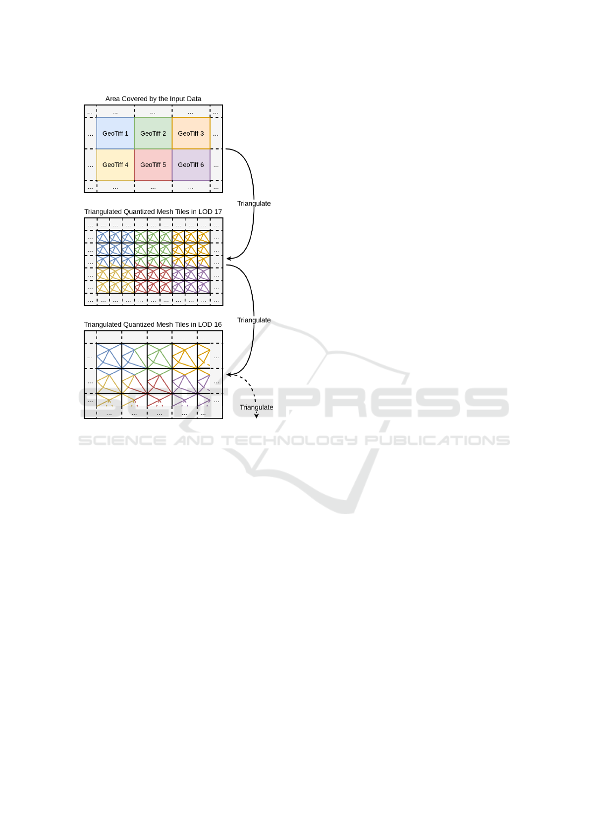
Figure 1: For each tile in the most accurate level (LOD 17

in this example), the required pixels are read from the input

GeoTiffs and triangulated. The resulting triangle meshes

are saved as quantized mesh ﬁles for each tile. These ﬁles

are ready for visualization. For a tile in LOD 16, we identify

the four tiles from LOD 17 on which it is based. We read

their vertices from the quantized mesh ﬁles and triangulate

them again with a coarser resolution. This is repeated until

we reach LOD 0 at the latest.

During LOD generation, we start at the most ac-

curate level. This level can be conﬁgured by the user

and should be selected depending on the resolution

of the input data. Figure 1 illustrates the process

with LOD 17 as most accurate level. We access the

GeoTiff ﬁles and compute the corresponding triangle

meshes. It is possible that a tile exceeds the bound-

aries of a GeoTiff. In this case, we read the required

pixels from multiple GeoTiff ﬁles. For example, this

applies to the tiles in the third row in Figure 1. We

store the triangulated tiles as quantized mesh ﬁles,

they are ready for visualization.

All other LODs are triangulated using the quan-

tized mesh ﬁles of the previous LOD as input. We

ﬁrst identify the four sub-tiles of the tile to be com-

puted. Then we access the corresponding quantized

mesh ﬁles and read the vertices from their triangle

meshes. These vertices are triangulated again, with

a higher allowed error. In this way, not all points are

used and the resolution of the new tile is lower. Fi-

nally, we save the new tile as a quantized mesh ﬁle

to make it available for the next coarser LOD and for

later visualization.

This approach has two major advantages: First,

the triangulation of the coarser levels is much faster,

since fewer points have to be considered. If we would

work on the original GeoTiff ﬁles instead, the coars-

est level would require reading the entire dataset. This

would take a lot of time and is not a practical solution.

Second, no separate data structure has to be stored be-

tween the LODs, because the quantized mesh ﬁles are

used directly. This saves I/O operations and speeds up

calculation.

3.2 Representation as a Scientiﬁc

Workﬂow

A scientiﬁc workﬂow consists of multiple tasks. They

may depend on each other if the outputs of one task

are needed as inputs for the other. In this case a se-

quential execution is necessary, otherwise the execu-

tion can be parallelized. The workﬂow management

system detects these dependencies and schedules the

execution in the cloud. We translated the terrain gen-

eration problem into the workﬂow illustrated in Fig-

ure 2.

As described above, the terrain data we generate

should be visualized in Cesium. For this, Cesium

needs a metadata ﬁle to know which tiles it can re-

quest. The ﬁle is created by our ﬁrst task called Cre-

ate Layers File. It takes the extent of the area to be

calculated, as well as the requested LODs and writes

the tiles to a JSON ﬁle. In addition, the task creates a

ﬁle in which the number of the highest, i.e. the most

accurate LOD is stored. This ﬁle is read by the second

task Generate Keys.

A naive approach for tile generation would be to

call the triangulation task for each tile in a LOD. In

theory, this approach enables maximum parallelism

since each tile could be generated simultaneously. In

practice, however, this parallelism would never be ex-

ploited. Even moderately large data sets lead to sev-

eral thousand tiles in the highest LOD. It is very un-

likely that so many VMs should be used and there-

fore, most of the tiles would be created one after the

other. Nevertheless, the workﬂow management sys-

tem would have to send a job to the VM for each tile

and receive the result. This adds unnecessary com-

munication overhead, which is why we introduced

batches.

Preprocessing of Terrain Data in the Cloud using a Workﬂow Management System

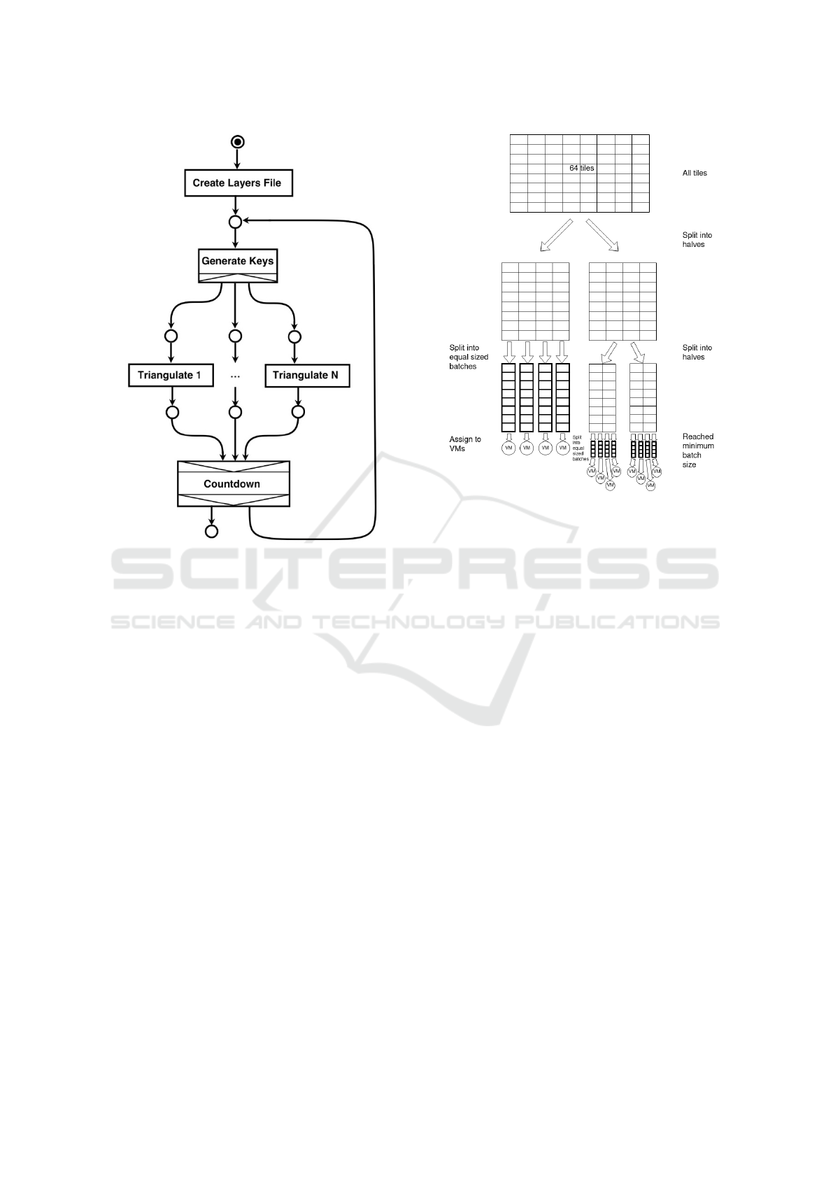
Figure 2: Workﬂow to generate a digital terrain model. Cre-

ate Layers File produces a metadata ﬁle for visualization,

Generate Keys groups multiple tiles into batches for a faster

processing and Triangulate calculates a triangle mesh for

each tile in a batch. Countdown iterates through all re-

quested level of detail and terminates the workﬂow when

completed.

The Generate Keys task groups the tiles of one

LOD into batches. As a result, the workﬂow man-

agement system will only distribute batches to the

VMs and not tiles. The batches should neither be too

large nor too small. If too few tiles are grouped, the

communication overhead will not be reduced. On the

other hand, the batches should not be too large ei-

ther. When a VM has ﬁnished processing its batch,

the workﬂow management system assigns a new one

to it. At some point all the batches of a LOD have

been distributed and it is necessary to wait for their

completion. The larger the batches, the more likely

it is that some VMs will ﬁnish considerably before

others. This reduces parallelism and slows down the

overall processing time.

An optimal batch size depends on the overhead for

executing a task, the number of VMs and the run time

of a process. These factors vary depending on the

used hardware and data. While it is possible to ﬁnd a

good batch size by trying different sizes, an automa-

tism would be favorable. We developed an algorithm

Figure 3: Grouping of tiles into batches. Each cell repre-

sents a tile. This example illustrates the grouping of 64 tiles

with 4 VMs and a minimum batch size of 4.

to deﬁne the batches automatically. It avoids a ﬁxed

batch size and instead varies the batch size during the

triangulation process. We start with large batches to

keep the VMs busy for a long time. Towards the end,

we use smaller batches. This enables us to react to

faster VMs and distribute remaining work more ﬂexi-

ble.

Figure 3 illustrates our grouping of tiles into

batches and their assignment to VMs. Generate Keys

splits the amount of tiles in two halves. The ﬁrst half

is distributed equally to all available VMs. This leads

to large batches so that many tiles can be calculated

with low communication overhead. The remaining

half of tiles is cut into halves again. Each new half

contains now a quarter of all tiles. The ﬁrst one is used

to generate as many batches as there are VMs again.

These new batches are smaller and enable the WMS

to react to different processing speeds of the VMs. To-

wards the end of the computation, this becomes more

important, which is why our batches are also getting

smaller. We continue halving and distributing the re-

maining tiles until the batch size is smaller than a se-

lected minimum. This minimum is the only conﬁgu-

ration the user has to provide. It can be set depending

on the performance of the VMs and the complexity of

the triangulation.

With our adaptive batch size, we can minimize the

communication overhead with the VMs and still as-

DATA 2022 - 11th International Conference on Data Science, Technology and Applications

sign new batches until the end. However, this ﬂexi-

bility must be supported by the WMS. In the imple-

mentation, a WMS has to be chosen that allows the

deﬁnition of tasks during run time.

When all batches for a LOD are processed, the

Countdown task reduces the LOD by one. Like Cre-

ate Layers File it creates a ﬁle in which the next LOD

is written down. This triggers the Generate Keys that

will group the tiles of this LOD to batches again.

When we reach the desired smallest LOD, Count-

down will not produce an output ﬁle and the workﬂow

terminates. The smallest LOD is at least 0 but can be

chosen higher if it makes sense for the input data.

4 EVALUATION

We evaluated our approach with the workﬂow man-

agement system Steep (Kr

amer, 2021). It supports

new tasks during run time and can be installed in a

cloud-based environment (Kr

amer et al., 2021).

As input data we used GeoTiff ﬁles, covering the

federal state of Hesse, Germany. Hesse has a total

area of approximately 20 thousand km

and our input

data consists of 973 ﬁles with a total size of 84 GB.

Each ﬁle has 5000 × 5000 pixels and a resolution of

one pixel per square meter. The data set is owned by

Hessian State Ofﬁce for Land Management and Geo-

Information (HVBG), a version with XYZ ﬁles in-

stead of GeoTiff is available as open data (Hessisches

Landesamt f

ur Bodenmanagement und Geoinforma-

tion, 2021).

In our evaluation we generate LOD 6 to 17.

LOD 17 is sufﬁcient to represent our highest resolu-

tion of one square meter. A coarser resolution than

LOD 6 does not make sense, because Hesse will be

too small in relation to the whole world. We calcu-

lated the LODs in a cloud-based environment (Sec-

tion 4.1) and examined the inﬂuence of various factors

on processing speed including parallelization (Section

4.2), the size of the batches (Section 4.3) and the in-

ﬂuence of the storage backend (Section 4.4).

4.1 Cloud Setup

The processing of the terrain data should be as efﬁ-

cient as possible. For this reason, we installed Steep

(version 5.9.0) in an OpenStack (Sefraoui et al., 2012)

cloud. Steep only starts VMs when there is something

to compute, afterwards they are shut down again.

Since terrain data only needs to be processed very ir-

regularly, such a setup reduces operating costs con-

siderably compared to a classic server solution.

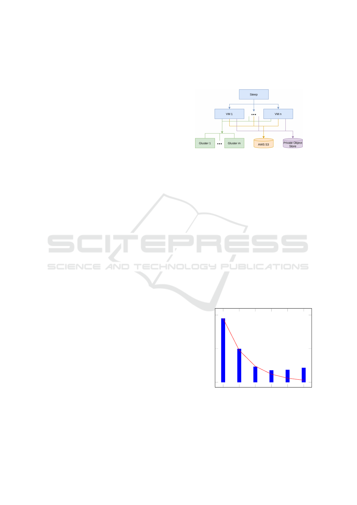
Our whole architecture is shown in Figure 4.

Steep itself is running on an instance with two cores

and 8 GB of RAM. When it receives a new workﬂow,

Steep starts new VMs to execute the tasks. These

VMs have 4 cores and 4 GB of RAM each.

Figure 4: System architecture.

The VMs have access to different storage back-

ends. The ﬁrst one is a distributed ﬁle system based

on GlusterFS (Red Hat Inc., 2019) and mounted us-

ing NFS. It is installed in the same OpenStack envi-

ronment than the other VMs and consists of multiple

instances with 2 cores, 8 GB memory and a hard disk.

Since the exact number of instances varies during our

evaluation, we will specify it with the measurements.

In Section 4.4 we will replace GlusterFS by AWS S3

(Amazon Web Services, Inc., 2021) as well as with a

private object store.

4.2 Parallelization

As mentioned in Section 4.1, our VMs have 4 cores.

We want to exploit them by computing multiple tiles

of a batch at the same time. For this we start several

threads on a VM. Each thread takes one tile from the

currently processed batch and computes it. When this

is done, it takes the next one until the whole batch is

1 2 4 8 16 32

1,000

2,000

1,897

991

459

351

365

425

Threads

Run time in minutes

Figure 5: Run time of 1 VM and 1 GlusterFS server with

different number of threads. Red line marks linear scaling.

Until 8 threads the run time decreases, afterwards it increase

again.

Preprocessing of Terrain Data in the Cloud using a Workﬂow Management System

processed. Figure 5 illustrates the inﬂuence of mul-

tiple threads on the total run time. An increase from

1 to 2 threads halves the run time. The same applies

to the change from 2 to 4 threads. This was expected,

since all cores of the VM are used in this way.

However, eight threads reduce the run time even

further before it increases again with 16 or more

threads. This can be explained by slower I/O oper-

ations. To compute a tile, the input data must be re-

trieved from the storage backend and the ﬁnished tile

has to be written back. Since all storage backends are

connected via the network, these I/O operations are

slow. By starting more threads than cores, we can hide

the I/O operations. While a thread waits for data, an-

other one can use the core for computation. However,

with 16 or more threads, the management overhead

dominates the beneﬁt, so the overall run time is nega-

tively affected. 8 threads are a good trade off between

management overhead and hiding I/O latency. We

will use this number for the following experiments.

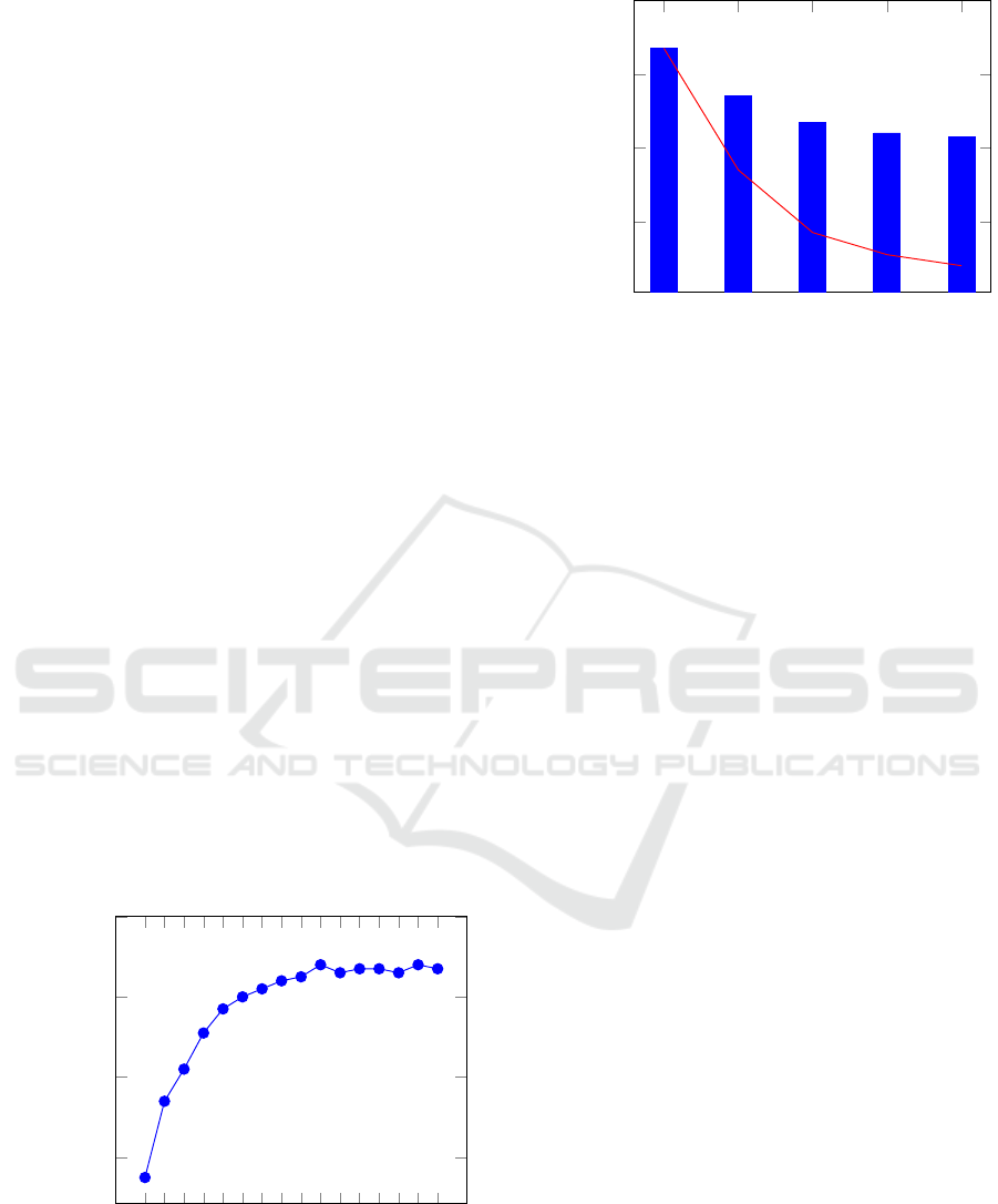
Besides parallelization through multiple threads,

we also use multiple VMs simultaneously. Figure 6

visualizes the run time for different numbers of VMs.

While one VM requires 351 minutes (this is the opti-

mum in Figure 5), additional VMs can further reduce

the run time. The process scales almost linearly with

up to 3 VMs but then starts to get slower the more

VMs are added. From about 10 VMs on, no consider-

able improvement can be observed.

Until now, all experiments used a single GlusterFS

server as storage backend. It is reasonable that this

storage becomes a bottleneck and increasing the num-

ber of VMs will not add any value. In Section 4.4, we

will therefore examine the storage backend in more

detail.

4.3 Batch Size

Our approach of an automatic varying of the batch

size aims to maximize the number of parallel working

1 2 3 4

5 6

7 8 9 10 11 12 13 14

15 16

100

200

300

400

351

183

134

107

71 71

69 69

VMs

Run time in minutes

Figure 6: Run time with one GlusterFS server and 8 threads.

Red line marks linear scaling.

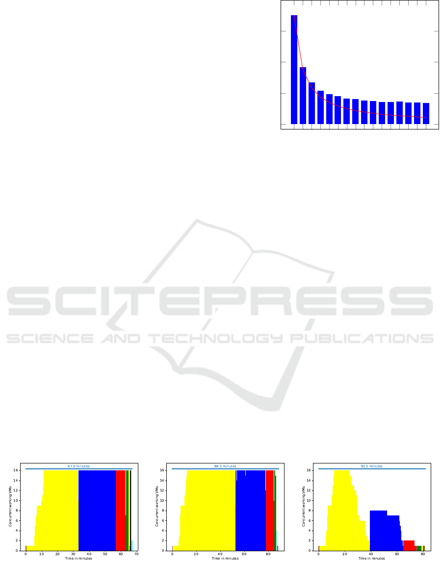
VMs. The VMs are created at run time. After a VM

is created, idling should be avoided and the communi-

cation overhead for batch distribution should be mini-

mized. Figure 7a visualizes how many of the 16 avail-

able VMs are created and running through the entire

triangulation process. Each color encodes a level of

detail, starting with the ﬁnest one in yellow.

The workﬂow starts with a single VM for the Cre-

ate Layers File and Generate Keys task. When the

triangulation of the batches starts, more VMs are cre-

ated. It takes about 13 minutes to start all 16 VMs.

When calculating LOD 17 (yellow), 16 (blue) and

15 (red) all VMs are working almost continuously.

In the coarser LODs the number of parallel work-

ing VMs is lower. In these levels, fewer tiles have to

be computed and it is no longer possible to generate

many long-running batches like in the ﬁrst LODs. As

mentioned in Section 3.2 the minimum batch size is a

trade off. If it is too small, the communication over-

head increases due to more scheduling effort. If it is

too large, there are not enough batches for all VMs.

In the last levels one of the problems always exists.

However, this applies only to a fraction of the total

(a) Our adaptive batch size. (b) Batch size 1 000. (c) Batch size 100 000.

Figure 7: Parallel running, i.e. non-idling VMs with 1 GlusterFS server, 8 threads and a maximum of 16 VMs. Color encodes

level of detail. (LOD 17 in yellow, LOD 16 in blue etc.) Brown bars encode another service than triangulate.

DATA 2022 - 11th International Conference on Data Science, Technology and Applications

processing time. Most of the time is needed for the

ﬁrst levels, that can be efﬁciently calculated by the

adaptive batch size.

We compared our approach to a ﬁxed batch size

of one thousand (Figure 7b) and 100 000 (Figure 7c).

One thousand tiles in a batch are too few. The VMs

are almost continuously utilized (similar to our ap-

proach), but the total run time is considerably higher

because of increased communication overhead. A

batch size of 100 000, on the other hand, is too large.

At the end of LOD 17 (yellow) there are not enough

batches left to keep all VMs busy. Starting with

LOD 16 (blue), some VMs are even idle from the be-

ginning. There are too few tiles to create such large

batches for all VMs. This again leads to a longer total

run time.

4.4 I/O Overhead

The GeoTiffs as well as the generated quantized mesh

ﬁles have to be stored somewhere. In the previous

sections, a single GlusterFS server was used for this

purpose. In Section 4.2, we assumed that increasing

the number of VMs does not improve performance

because the storage backend is the bottleneck. This

assumption is supported when looking at the CPU

load of the GlusterFS instance (Figure 8). It reaches

an upper bound of almost 90% for more than 10 VMs.

This indicates that the one GlusterFS server is not able

to provide more than 10 VMs with data.

In this section, we examine the impact of addi-

tional GluserFS servers on the overall run time. To

provide better comparability of our work, we also re-

placed GlusterFS with AWS S3, as well as with a pri-

vate object storage.

1 2 3 4

5 6

7 8 9 10 11 12 13 14

15 16

100

VMs

Average CPU utilization

Figure 8: Average CPU utilization of the single GlusterFS

server during triangulation with varying number of VMs

and 8 threads each.

1 2 4 6 8

GlusterFS server

Run time in minutes

Figure 9: Run time with 16 VMs, 8 threads and a varying

amount of GlusterFS servers. Red line marks linear scaling.

GlusterFS Servers

In the previous experiments, we ﬁxed the number of

GlusterFS servers to 1. Now we add more GlusterFS

server in the distributed volume mode. In this way

a ﬁle is stored on just one server without replication.

Due to their random distribution, each server has a

similar workload during the calculation.

We calculated the LODs again with 16 VMs and

8 threads each, but varied the number of GlusterFS

servers (Figure 9). As expected, more GlusterFS

servers reduce run time. However, the speedup is sig-

niﬁcantly less than it was for more threads or VMs.

The difference to a linear scaling is already clearly

visible when switching from one to two GlusterFS

servers. Nevertheless, the run time can be improved

by another 35% with 8 GlusterFS servers compared

to just one.

AWS S3

To assure compatibility of our results, we run the

same experiment (16 VMs, 8 threads) with Amazon

AWS S3 instead of GlusterFS. The run time is 184

minutes and therefore much slower than with one

GlusterFS server (67 minutes). While S3 itself pro-

vides fast storage access, the latency is higher due

to the higher physical distance between the servers.

In addition, the large number of small ﬁles results in

many read and write operations. These are charged

by AWS, leading to higher operating costs.

Private Object Store

We repeat the same experiment with a private object

store. It uses the same access protocol than AWS S3

but the servers are closer to our cluster. This improves

Preprocessing of Terrain Data in the Cloud using a Workﬂow Management System

the run time from 184 minutes (AWS S3) to 108 min-

utes an conﬁrms the great inﬂuence of I/O latency.

5 COMPARISON WITH

PREVIOUS WORK

In our previous work we performed the same task

on the same data set but used GeoTrellis on top of

Apache Spark instead of a workﬂow management

system (Kr

amer et al., 2020). As mentioned above,

this approach had the advantage of being easy to set

up. However, the frameworks limited us and led to

undesired behavior such as resampling of input data

and many shufﬂe operations during processing. With

our new approach we want to circumvent this and in-

crease the performance considerably.

In our previous work we had 16 GlusterFS servers

with 2 cores and 8 GB of RAM. On these instances,

the LODs were calculated as well. This differs from

our new approach, where the instances for calculating

are separated from those for storing the data.

Our total run time with the old approach is

79 hours when using 16 instances for GlusterFS in-

cluding one for calculating the LODs. The new ap-

proach needs less than 6 hours with a single GlusterFS

instance combined with one for calculation. This is a

huge improvement of factor 13 even considering that

we now used 4 cores instead of 2. Our best run time

in the old approach used 15 calculating VMs and took

354 minutes. The new approach is 5 times faster with

67 minutes. If we add ﬁve more GlusterFS servers we

can even reduce the run time to 44 minutes.

These measurements conﬁrm that our new ap-

proach brings signiﬁcant performance improvements.

It is superior to the old approach and demonstrates

that workﬂow management systems are a powerful

basis for the processing of terrain data.

6 CONCLUSION

In this paper, we computed the LODs for a terrain

model using a scientiﬁc workﬂow. During calcula-

tion we used the results from a more accurate LOD to

speed up the computations of the next coarser LOD.

Since we used already generated data, we did not need

an additional data structure. This saved I/O operations

and sped up calculation.

However, we store each resulting tile as an indi-

vidual ﬁle. For the data set used, this is about 2.5 mil-

lion ﬁles with a few kilobytes each. In a future work

we want to combine all tiles of a batch in one large

ﬁle. This would reduce the number of I/O operations

and speed up calculation further. In addition, the costs

of AWS S3 are calculated based on the number of data

accesses. Reducing the number of ﬁles reduces oper-

ating costs when using AWS S3 as a storage backend.

The drawback of this solution is that the byte ranges

of the individual tiles must be captured. If a tile is

read, only these bytes have to be returned from the

larger ﬁle. Nevertheless, this is a promising approach

that should be investigated in future work.

In our approach, the WMS starts VMs for the cal-

culations. This provides a lot of ﬂexibility, but we

have to wait a few minutes before newly started VMs

are ready. In the future, we want to explore the possi-

bilities of serverless computing. Instead of launching

VMs, the WMS could run containers directly through

the cloud provider. In this way, the infrastructure

would be further simpliﬁed and new types of orches-

tration would be possible.

Our main contribution in this paper is the prepara-

tion of terrain data using a scientiﬁc workﬂow. For

this purpose, we introduced an adaptive batch size

that bundles several tiles in one batch. The dynamic

size of these batches enables the workﬂow manage-

ment system to consistently utilize all available VMs,

minimizing their idle time and speed up the calcula-

tion.

Our evaluation shows that our approach scales

well when computation power is added. With

16 VMs, we can prepare the entire test data set in

just over an hour, while it takes almost six hours on

a single instance. This is signiﬁcantly faster than our

previous work, where we needed 15 VMs to process

the data set in under six hours.

With our new approach, even large data sets can

be prepared for visualization efﬁciently. The required

VMs are started on demand and are continuously used

afterwards. This leads to fast results and low operat-

ing costs at the same time.

REFERENCES

Agarwal, D. (2012). Crayons : An Azure Cloud based

Parallel Sy stem for GIS Overlay Operations. page

1048200.

Alonso, G. and Hagen, C. (1997). Geo-opera: Work-

ﬂow concepts for spatial processes. In International

Symposium on Spatial Databases, pages 238–258.

Springer.

Amazon Web Services, Inc. (2021). Amazon simple stor-

age service s3 – cloud online-speicher. https://aws.

amazon.com/de/s3/. accessed 08-Dec-2021.

Apache Software Foundation (2021). Apache hadoop.

https://hadoop.apache.org/. accessed 09-Aug-2021.

DATA 2022 - 11th International Conference on Data Science, Technology and Applications

Azavea Inc. (2021). Geotrellis. https://geotrellis.io/. ac-

cessed 09-Aug-2021.

Beisken, S., Meinl, T., Wiswedel, B., de Figueiredo, L. F.,

Berthold, M., and Steinbeck, C. (2013). Knime-cdk:

Workﬂow-driven cheminformatics. BMC bioinfor-

matics, 14(1):1–4.

Berriman, G. B., Deelman, E., Good, J. C., Jacob, J. C.,

Katz, D. S., Kesselman, C., Laity, A. C., Prince, T. A.,

Singh, G., and Su, M.-H. (2004). Montage: a grid-

enabled engine for delivering custom science-grade

mosaics on demand. In Optimizing scientiﬁc return

for astronomy through information technologies, vol-

ume 5493, pages 221–232. SPIE.

Cesium GS, Inc. (2022). Cesium: The platform for 3d

geospatial. https://cesium.com. accessed 03-Feb-

2022.

CesiumGS (2020). Geotiffquantized-mesh. https://github.

com/CesiumGS/quantized-mesh. accessed 28-Sep-

2021.

Crawl, D., Block, J., Lin, K., and Altintas, I. (2017).

Firemap: A dynamic data-driven predictive wildﬁre

modeling and visualization environment. Procedia

Computer Science, 108:2230–2239.

Cui, D., Wu, Y., and Zhang, Q. (2010). Massive spatial data

processing model based on cloud computing model.

3rd International Joint Conference on Computational

Sciences and Optimization, CSO 2010: Theoretical

Development and Engineering Practice, 2:347–350.

De Berg, M., Cheong, O., Van Kreveld, M., and Overmars,

M. (2008). Computational geometry: Algorithms and

applications. Computational geometry: algorithms

and applications, pages 1–17.

Dean, J. and Ghemawat, S. (2008). Mapreduce: Simpli-

ﬁed data processing on large clusters. Commun. ACM,

51(1):107–113.

Delaunay, B. et al. (1934). Sur la sphere vide. Izv. Akad.

Nauk SSSR, Otdelenie Matematicheskii i Estestven-

nyka Nauk, 7(793-800):1–2.

Du, Y. and Cheng, P. (2017). Lwgeowfms: A lightweight

geo-workﬂow management system. In IOP Confer-

ence Series: Earth and Environmental Science, vol-

ume 59, page 012070. IOP Publishing.

Giachetta, R. (2015). A framework for processing large

scale geospatial and remote sensing data in MapRe-

duce environment. Computers and Graphics (Perga-

mon), 49:37–46.

Hegeman, J. W., Sardeshmukh, V. B., Sugumaran, R., and

Armstrong, M. P. (2014). Distributed LiDAR data pro-

cessing in a high-memory cloud-computing environ-

ment. Annals of GIS, 20(4):255–264.

Hessisches Landesamt f

ur Bodenmanagement und Geoin-

formation (2021). Hessian geodata portal: Geodaten

online. https://www.gds.hessen.de. accessed 08-Dec-

2021.

Hughes, J. N., Annex, A., Eichelberger, C. N., Fox, A.,

Hulbert, A., and Ronquest, M. (2015). GeoMesa:

a distributed architecture for spatio-temporal fusion.

In Pellechia, M. F., Palaniappan, K., Doucette, P. J.,

Dockstader, S. L., Seetharaman, G., and Deignan,

P. B., editors, Geospatial Informatics, Fusion, and

Motion Video Analytics V, volume 9473, pages 128

– 140. International Society for Optics and Photonics,

SPIE.

amer, M. (2021). Efﬁcient scheduling of scientiﬁc work-

ﬂow actions in the cloud based on required capabil-

ities. In Hammoudi, S., Quix, C., and Bernardino,

J., editors, Data Management Technologies and Ap-

plications, pages 32–55, Cham. Springer International

Publishing.

amer, M., Gutbell, R., W

urz, H. M., and Weil, J. (2020).

Scalable processing of massive geodata in the cloud:

generating a level-of-detail structure optimized for

web visualization. AGILE: GIScience Series, pages

1–20.

amer, M., W

urz, H. M., and Altenhofen, C. (2021). Ex-

ecuting cyclic scientiﬁc workﬂows in the cloud. Jour-

nal of Cloud Computing, 10(1):1–26.

Larsonneur, E., Mercier, J., Wiart, N., Floch, E., Del-

homme, O., and Meyer, V. (2018). Evaluating work-

ﬂow management systems: A bioinformatics use case.

pages 2773–2775.

Maptools.org (2020). Geotiff. http://geotiff.maptools.org/

spec/contents.html. accessed 28-Sep-2021.

Medeiros, C. B., Vossen, G., and Weske, M. (1996). Geo-

wasa-combining gis technology with workﬂow man-

agement. In Proceedings of the Seventh Israeli Con-

ference on Computer Systems and Software Engineer-

ing, pages 129–139. IEEE.

Oinn, T., Greenwood, M., Addis, M., Alpdemir, M. N.,

Ferris, J., Glover, K., Goble, C., Goderis, A., Hull,

D., Marvin, D., Li, P., Lord, P., Pocock, M. R., Sen-

ger, M., Stevens, R., Wipat, A., and Wroe, C. (2006).

Taverna: lessons in creating a workﬂow environment

for the life sciences. Concurrency and Computation:

Practice and Experience, 18(10):1067–1100.

Open Source Geospatial Foundation (2012). Tile map ser-

vice speciﬁcation. https://wiki.osgeo.org/wiki/Tile

Map Service Speciﬁcation. accessed 08-Dec-2021.

Red Hat Inc. (2019). Gluster. https://gluster.org. accessed

28-Sep-2021.

Sefraoui, O., Aissaoui, M., and Eleuldj, M. (2012). Open-

stack: toward an open-source solution for cloud com-

puting. International Journal of Computer Applica-

tions, 55(3):38–42.

Wang, Y., Liu, Z., Liao, H., and Li, C. (2015). Improving

the performance of GIS polygon overlay computation

with MapReduce for spatial big data processing. Clus-

ter Computing, 18(2):507–516.

Zaharia, M., Chowdhury, M., Franklin, M. J., Shenker, S.,

Stoica, I., et al. (2010). Spark: Cluster computing with

working sets. HotCloud, 10(10-10):95.

Zhong, Y., Han, J., Zhang, T., and Fang, J. (2012). A

distributed geospatial data storage and processing

framework for large-scale WebGIS. Proceedings -

2012 20th International Conference on Geoinformat-

ics, Geoinformatics 2012, (20).

Preprocessing of Terrain Data in the Cloud using a Workﬂow Management System