Performance Analysis of an Embedded System for Target Detection

in Smart Crosswalks using Machine Learning

J. M. Lozano Domínguez

, J. M. Corralejo Mora

, I. J. Fernández de Viana González

T. J. Mateo Sanguino

and M. J. Redondo González

Department of Electronic Engineering, Computer Systems and Automatics, University of Huelva,

Av. de las Artes s/n, 21007 Huelva, Spain

Department of Information Technologies, University of Huelva, Av. de las Artes s/n, 21007 Huelva, Spain

Keywords: Embedded System, Machine Learning, Performance Analysis, Road Signalling, Target Detection.

Abstract: Embedded systems with low computing resources for artificial intelligence are being a key piece for the

deployment of the Internet of Things in different areas as energy efficiency, agriculture or water monitoring,

amid others. This paper carries out a study of the computational performance of a smart road detection and

signalling system. To this end, the implementation methodology from Matlab

to C++ of a one-class SVM

classifier with two pattern analysis strategies based on RADAR signals and RAW data is described. As a

result, we found a balance between AUC, RAM consumption, processing time and power consumption for a

Teensy 4.1 microcontroller with STFT and the fitcsvm2 algorithm versus other hardware options such as an

I7-3770K processor, Raspberry Pi Zero and Teensy 3.6.

1 INTRODUCTION

In recent years, there has been a boom of the Internet

of Things (IoT) devices, which are embedded systems

that incorporate specific software to work in different

fields of application (Zanella, 2014). These areas

include energy efficiency (Alowaidi, 2022),

agriculture (Rahman, 2022) or water treatment

monitoring (Sugamar, 2021) among others.

The increasing improvement of IoT devices has

made it possible to include machine learning (ML)

algorithms in control units with scarce computational

resources, such as microcontrollers (Gopinath, 2019).

As an example, a comparison of machine learning

techniques was carried out to minimize water loss

during irrigation operations (Amassmir, 2022). In this

work, Raspberry Pi 3 is used as a control unit in which

an artificial neural network (ANN) was the technique

that offered the best performance. Another work

includes the use of support vector machines (SVM) to

detect cardiac anomalies in patients through

characteristics extracted from a fast Fourier transform

https://orcid.org/0000-0002-2542-0517

https://orcid.org/0000-0002-9689-8884

https://orcid.org/0000-0002-9387-3892

https://orcid.org/0000-0001-5550-1310

(FFT). In this case, a 32-bit microcontroller system

was used to implement the machine learning

technique, achieving an accuracy of up to 95.68%

(Raj, 2020). There are also cases in the field of road

safety where a solution for accident detection and

classification alerts emergency systems based on the

severity of the accident (Balfaqih, 2022). For this, the

techniques named Gaussian Mixture Model (GMM)

and Classification and Regression Trees (CART)

were integrated into an Arduino Mega. Other work

proposed the use of ML techniques to detect

anomalies in traffic data to dynamically regulate road

signs. This solution was implemented on Raspberry

Pi 3 (Sankaranarayanan, 2019).

This paper describes an improvement of a road

detection and signalling system aimed at

distinguishing road targets through sensory fusion

and fuzzy logic (Lozano Domínguez, 2018).

Specifically, when a pedestrian is detected on a

crosswalk, the system generates visual cues that alert

drivers to stop their vehicle safely. With this purpose,

another approach for target detection using RADAR

382

Lozano Domínguez, J., Corralejo Mora, J., Fernández de Viana González, I., Mateo Sanguino, T. and Redondo González, M.

Performance Analysis of an Embedded System for Target Detection in Smart Crosswalks using Machine Learning.

DOI: 10.5220/0011142700003266

In Proceedings of the 17th International Conference on Software Technologies (ICSOFT 2022), pages 382-389

ISBN: 978-989-758-588-3; ISSN: 2184-2833

sensors and signal analysis applying Short Time

Fourier Transform (STFT) on a PC was investigated

(Domínguez, 2020). Furthermore, a vehicle detection

system based on ML techniques was tested for a smart

pedestrian crosswalk (Lozano Domínguez, 2021).

The current work aims to combine the previous works

on STFT analysis and vehicle detection to apply them

to an embedded system focused on discerning

pedestrians by detecting signal patterns through ML

techniques. The goal here is to validate a generic

methodology —without a domain-specific language

as in (Gopinath, 2019)

—

to implement ML

algorithms in a constrained microcontroller while

performing more costly pre-processing tasks (i.e.,

STFT) than the classification task itself. To do this,

the paper presents the implementation of several ML

techniques in an embedded system with a greater

limitation of RAM memory, CPU speed and power

consumption than other state-of-the-art solutions

based on Raspberry Pi or FPGA.

This manuscript has been structured as follows:

Section 2 describes the hardware and software of the

embedded system implemented to classify

pedestrians. Section 3 presents the ML algorithm

used, the implementation into a microcontroller and

the experimentation carried out. Finally, Section 4

highlights the conclusions and future work.

2 SYSTEM DESCRIPTION

This section describes the main hardware

components, the AI techniques applied to detect

different targets and, finally, the methodology

followed to extract a ML model and translate it into

C++ code to be interpreted by a microcontroller unit.

2.1 Hardware Components

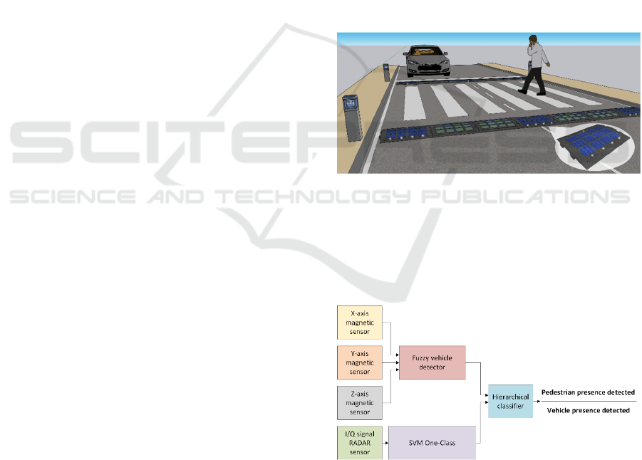
The road signalling system is made up of a set of

intelligent nodes ubicated in the limits of a crosswalk,

each one covering an area (Fig. 1). The nodes

integrate sensors facing the inner and outer faces of

the crosswalk to detect nearby objects. A traffic-

oriented illumination is activated when pedestrians

are detected in the zebra crossing. Then, the detector

node handles the communication with the rest of the

network to synchronize the flashing lights and thus

improve road safety.

Each node integrates a microcontroller, wireless

communication, sensors, signalling and power unit.

We selected a Teensy 4.1 device to analyse data

sensor periodically collected, identify the target type

and activate the signalling unit when necessary. The

latter is composed by four high brightness white

LEDs oriented to oncoming drivers (Lumileds L128-

5070HA) and one amber LED oriented to pedestrians

(Lumileds L128-PCA12500000). The sequence and

brightness of the LEDs is controlled with a blinking

pattern through pulse width modulation (PWM). The

communication unit is implemented with a Microchip

ATSAMR21B18 device compliant with the IEEE

802.15.4 standard in an effort to save energy. The

detection unit combines Doppler RADARs and a

magnetic sensor. To this end, we selected two

RFbeam Microwave GmbH K-LD7 devices in the

24GHz band, one oriented to detect bicycles and cars,

and the other oriented to detect pedestrians.

Moreover, a STMicroelectronics LIS3MDL magnetic

sensor is used to complementarily detect the presence

of vehicles. Finally, the power unit supplies energy to

the system through a Texas Instruments

BQ25895RTWR charger connected to a set of solar

panels and Lithium Polymer (LiPo) batteries.

Figure 1: Overall diagram of the smart crosswalk.

2.2

Software Description

To detect and distinguish between vehicles and

pedestrians on a crosswalk, the developed software

follows the data flow described in Figure 2.

Figure 2: Software system structure.

The RADARs provide an I/Q signal containing

the speed and pattern information of the targets in

relation to their Doppler frequency. The control unit

processes this signal through the STFT, which allows

performing a spectral analysis of the signal. The

Performance Analysis of an Embedded System for Target Detection in Smart Crosswalks using Machine Learning

383

signal pattern is used to feed the characteristics of the

ML algorithm and identify different targets such a

walking person or a vehicle (Domínguez, 2020). To

this end, the system merges data generated in the

different sensors in a sensory fusion process. On the

one hand, the one-class support vector machine

(SVM) has been implemented to process data from

the RADARs, separately. On the other hand, a fuzzy

logic process has been developed to analyse the

magnetic sensor data. This estimates the presence of

vehicles depending on detected perturbations and can

be auto calibrated to detect even stopped vehicles. In

this way, when the one-class SVM determines the

presence of a pedestrian on the crosswalk and the

diffuse vehicle detector does not detect the presence

of vehicles, the system takes a decision through a

hierarchical classifier based on traditional logic. In

this way, the entire system activates the signalling

units in the presence of pedestrians in the vicinity of

the crosswalk. In this section, the details related to the

AI techniques used in the system will be exposed.

2.2.1 Implementation of Fuzzy Logic to

Detect Vehicles

The block called “Fuzzy vehicle detector” is used to

determine the presence or absence of vehicles around

a crosswalk by changes in the magnetic field. These

perturbations are produced due to the presence of

ferromagnetic elements in vehicles, whose values are

measured on the X, Y, and Z axes. The vehicle

detector block is a Mamdani-type fuzzy rule-based

controller with classification norms such as “If X

and … Xn is Xn, then Y is B” (Mamdani, 1977).

Both, the predictor and output variables have been

established by an expert system. To this end, we used

trapezoidal functions to establish the membership of

a fuzzy set since the adequacy to the data model is

correct and computationally simple. In addition, the

conjunction and implication operators used the

minimum T-norm (Aliev, 2013). The defuzzification

process uses the FITA method (i.e., First Inter, Then

Aggregate) in contrast to the less consistent FATI

method (Ibrahim, 2004). The process also used the

MVP weighting method (Buckley, 1994).

The vehicle detector has three inputs (i.e., one per

axis) with three tags named Changeα, NoChangeα

and ChangeNα, where α means the corresponding

axis. NoChangeα stands for the value of the magnetic

field during the idle state of the sensor, while

Changeα and ChangeNα mean a magnetic field

variation below and above the idle state, respectively.

The output of the magnetic controller ranges between

0-1 to indicate absence or presence of vehicles close

to a crosswalk (i.e., No and Yes). The rules base and

tags of the magnetic controller were experimentally

stablished by the expert system as shown in Table 1.

Accordingly, it was established that a variation of the

idle state of the magnetic sensor in at least 2/3 of its

axes indicates the presence of vehicles circulating on

the crosswalk. In another case, this means that the

vehicles do not exist.

In addition to the fuzzy rule base, a logic that takes

the last five results of the magnetic controller is

considered. If one of these five values exceeds the

threshold of belonging to the vehicle set called “Yes”

above 0.5, the presence of a vehicle is determined.

Said logic also considers that, if after a minute in

which the values of the vehicle presence are detected

continuously, the diffuse labels of the magnetic

sensor are recalibrated because this may be caused by

a vehicle parked near the crosswalk. This approach

has been implemented directly in C++ through

classes and interfaces.

Table 1: Rule base for the magnetic fuzzy controller.

Label x-axis Label y-axis Label z-axis Vehicle

NoChangeX NoChangeY NoChangeZ No

NoChangeX NoChange ChangeNZ No

NoChangeX NoChangeY NoChangeZ No

NoChangeX ChangeNY NoChangeZ No

NoChangeX ChangeNY ChangeNZ Yes

NoChangeX ChangeNY NoChangeZ Yes

NoChangeX ChangeY NoChangeZ No

NoChangeX ChangeY ChangeNZ Yes

NoChangeX ChangeY NoChangeZ Yes

ChangeNX NoChangeY NoChangeZ No

ChangeNX NoChange ChangeNZ Yes

ChangeNX NoChangeY NoChangeZ Yes

ChangeNX ChangeNY NoChangeZ Yes

ChangeNX ChangeNY ChangeNZ Yes

ChangeNX ChangeNY NoChangeZ Yes

ChangeNX ChangeY NoChangeZ Yes

ChangeNX ChangeY ChangeNZ Yes

ChangeNX ChangeY NoChangeZ Yes

ChangeX NoChangeY NoChangeZ No

ChangeX NoChange ChangeNZ Yes

ChangeX NoChangeY NoChangeZ Yes

ChangeX ChangeNY NoChangeZ Yes

ChangeX ChangeNY ChangeNZ Yes

ChangeX ChangeNY NoChangeZ Yes

ChangeX ChangeY NoChangeZ Yes

ChangeX ChangeY ChangeNZ Yes

ChangeX ChangeY NoChangeZ Yes

ICSOFT 2022 - 17th International Conference on Software Technologies

384

2.2.2 Implementation of One-class to Detect

Pedestrians

One-class SVM is an unsupervised ML technique that

has been implemented in Matlab

with the “fitcsvm”

library. This technique allows detecting outliers or

anomalies in the analyzed data, as well as training

with only one target class that, in our case, it would

be pedestrians. In this way, pedestrians are the targets

of the main class while vehicles and the idle state are

considered outliers. This approach has been preferred

because the only targets that should generate a light

alert are pedestrians, whilst any target that does not

have the characteristics of a pedestrian will not cause

an activation. The main advantage of this ML

technique over others is that only the “pedestrian”

class needs to be known to be trained. Furthermore, it

offers good handling of unbalanced classes and is

very sensitive to outliers. On the contrary, it requires

a good selection of hyperparameters and kernels by

the expert system (Singla, 2020).

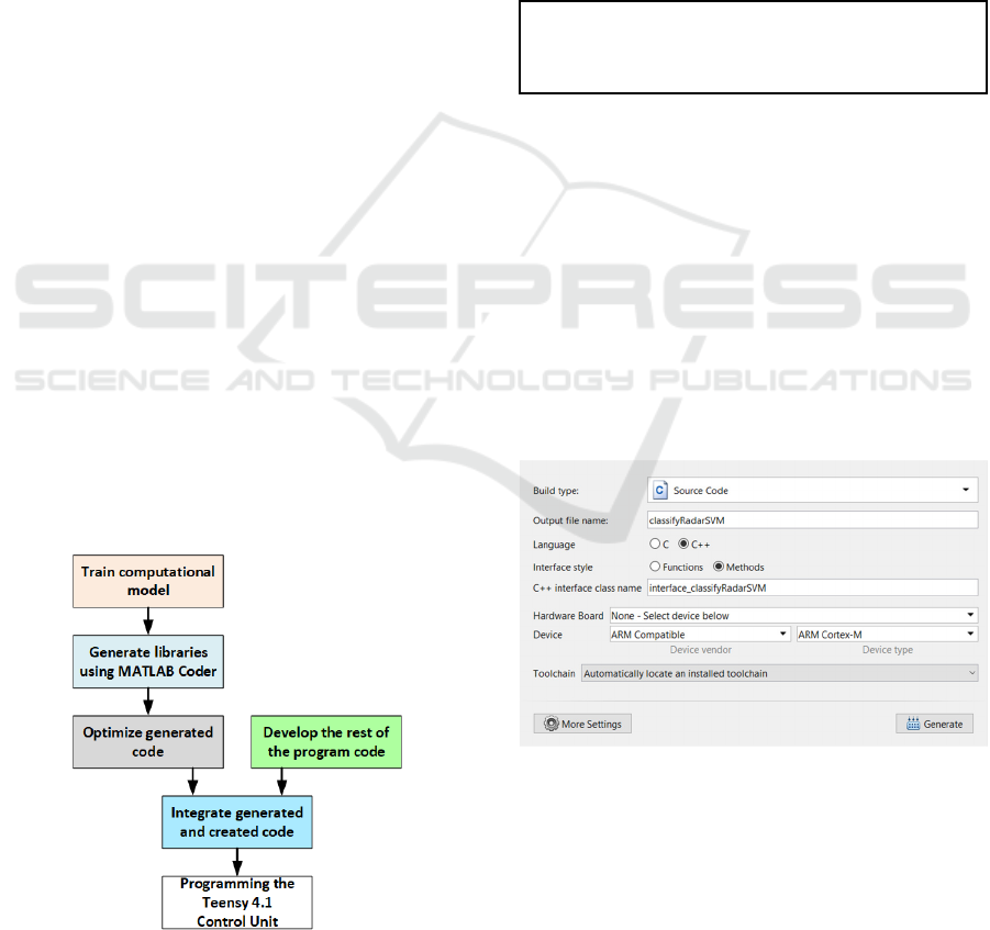
2.3

Conversion from Matlab to C++

This section describes the steps followed to export the

ML model generated after training the algorithm from

Matlab

to C++ code. The process is summarized in

Figure 3. The C++ language has been selected

because it is the one used in the integrated

development environment (IDE) to generate the

binary code of the control unit used (i.e., Teensy 4.1).

The procedure followed has been: i) generate a

Matlab

script with the necessary functions for the

execution of the program; ii) configure the Matlab

Coder tool to generate the code optimally; and iii)

perform an optimization of both the variables and the

code autogenerated by Matlab

Figure 3: Code conversion procedure.

Firstly, the script to be created in Matlab

must

contain the same number of inputs as those used by

the ML model, as well as specify the processing of

these inputs, if any. On the one hand, it is necessary

to specify that the model must be loaded through the

“loadLearnerForCoder” function, which allows

generating the automatic learning models in C/C++

code. On the other hand, the “predict” function must

be used to obtain the classifier’s prediction based on

the inputs (i.e., features obtained from the normalized

STFT). Finally, the output generated by the model

must also be added (i.e., pedestrian presence). The

script used can be seen in Algorithm 1.

Algorithm 1: Function to generate the ML model.

function output= classifyRadarSVM(inputs)

Mdl = loadLearnerForCoder('Model Name');

output= predict(Mdl,X);

Second, the Matlab Coder tool is required to

generate the C/C++ code from the previously

described script. This tool allows selecting whether

the source code to be generated will be C or C++,

define the name of the interfaces and select the

hardware on which the code is going to be executed

to optimize it. In the present case, none has been

selected in "Hardware Board" and then it has been

indicated that the microcontroller belongs to the

ARM Cortex-M family (Figure 4). Furthermore, it

has been indicated in the tool configuration that the

OpenMP library cannot be used, since our

microcontroller only has one processing thread.

Figure 4: Matlab Coder configuration.

Finally, an optimization of the libraries generated

by this tool was performed to adapt them to the

hardware used and reduce the space occupied in

memory. For this, the code has been analyzed in

search of possible duplications of temporary variables

in memory. Furthermore, it has been sought that those

variables initialized in their declaration remain

Performance Analysis of an Embedded System for Target Detection in Smart Crosswalks using Machine Learning

385

resident in memory to avoid copy operations during

periodic execution. The variables most frequently

accessed have been allocated in the fastest memory

areas.

The optimized code is included in the project as

part of a functional module, which is called periodically

to classify the RADAR signal.

3 EXPERIMENTATION

The K-LD7 sensor provides two types of signals. On

the one hand, PDAT provides an array of RAW data

with the speed, angle, distance and magnitude of the

targets detected. On the other hand, the RADAR

provides the I/Q signal to be later processed to obtain

identifying characteristics of the targets.

Accordingly, this section will detail the steps

followed to process the I/Q signal as the main method

to obtain additional features to those provided by the

PDAT signal.

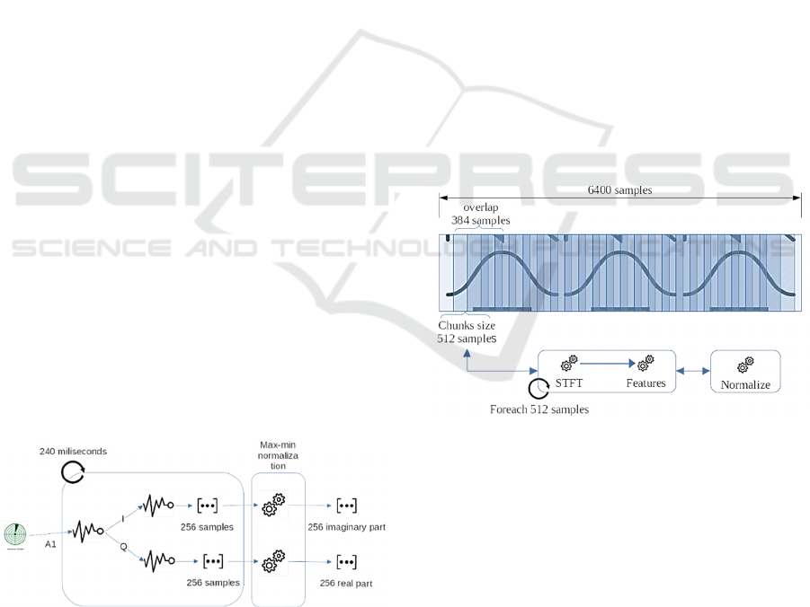
3.1 Data Pre-processing

The process begins by acquiring the A1 signal from

the K-LD7 sensor, which refers to the signal reflected

by frequency A of the RADAR received at antenna 1.

Signal A1 is a composite I/Q signal (i.e., “in phase”

and “in quadrature”), thus standing for the real and

imaginary values conforming the signal. These

signals are obtained in sets of 256 values taken with a

sampling frequency of 1100 Hz. To do this, the

RADAR query period was set to 240ms so that it was

the minimum time needed to store and communicate

a 256-value sample (see actual CPU usage in Tables

5 and 6). Once the signals are obtained, they are

normalized separately using the Min-Max method

since it is a suitable method to be the training base for

ML algorithms (Al Shalabi, 2006). This process is

depicted in Figure 5.

Figure 5: I/Q signal acquisition process.

To obtain the data to train and test the classifiers,

an outdoor setup where the RADAR captured several

scenes involving vehicles and pedestrians was

established. These included vehicles approaching,

moving away, stopping and starting, as well as

individuals, groups of people, pedestrians with pets,

cyclists and scooter users. Figure 6 details the steps

followed to process each of the scenes. Each one is

made up of 25 consecutive RADAR acquisitions,

giving us a total of 6400 samples per scene.

Subsequently, the real and imaginary parts of the

signal were processed by means of the STFT.

Specifically, we applied a sample rate of 1100 Hz, a

Kaiser-type window, an overlap length of 200 values

and an FFT size of 512 points. Then, it was divided

into chunks made up of the same number of points.

Each one of these pieces are the minimum units to be

classified. That is, the labels of the classification

process will be assigned to these pieces and not to

each one of the samples that form them.

Preliminary tests were carried out to obtain the

minimum cut-off size that optimizes the classification

results in relation to the space used to store the signal.

Amid different sizes (i.e., from 256 to 8192 values),

it was found that the best results were achieved with

512 values, whilst sizes greater than 2048 were

discarded due to hardware restrictions. In addition,

and in order not to lose the temporal evolution of the

signal, it was decided to chop the signal with an offset

of 128 values. Therefore, each of the scenes is divided

into 50 pieces.

Figure 6: Overview of a scene processing.

The next step was to characterize each of the

pieces obtained. For each one, 20 features were

obtained based on simple statistical calculations such

as the mean value, variance, difference between the

maximum and minimum value, median or the

kurtosis value. Finally, the feature values were

normalized by the Euclidean norm (i.e., 2-norm).

Table 2 shows the whole list of features.

Once the scenes were characterized, the next step

was their labelling by a group of experts. As said

before, each piece is labelled independently. The

strategy followed by the experts was to assign the

target label ‒represented by 1‒ when the crosswalk

ICSOFT 2022 - 17th International Conference on Software Technologies

386

must light up the LEDs and the outlier label ‒

represented by 0‒ in other cases. For the experiments

performed in this paper, a total of 81 scenes were

defined resulting in a total of 4050 labelled chunks.

Table 2: Features applied to extract the STFT pattern.

Features #1-10 Features #11-20

mean(sliceVec); median(sliceVec)

mean(sliceVec.^2) mean(std(slice,0,1)

mean(sliceVec.^3) std(mean(slice,1))

mean(sliceVec.^4) std(std(slice))

std(sliceVec); std(std(slice,0,1))

skewness(sliceVec); mean(std(slice,0,2)

kurtosis(sliceVec); std(mean(slice,2))

quantile(sliceVec,0.25) std(std(slice))

quantile(sliceVec,0.50) std(std(slice,0,2))

quantile(sliceVec,0.75) max(sliceVec)-min(sliceVec)

3.2 Parameter Settings and Learning

Outcomes

Two different datasets were used to study the

behaviour of the one-class SVM classifier. The first

one was formed by the data obtained from the PDAT

signal and the second one by the data obtained after

processing the I/Q signals (see Section 3.1). The one-

class SVM classifier used in this paper applies the

radial basis kernel, find a scale value for the kernel

function and standardize the predictors. These values

were not tuned because, apart from being far from the

goals of this paper, very promising results were

obtained. In addition to the one-class SVM classifier,

we tested other one-class classifiers provided by the

ddtools library as well as bi-class classifiers such as

TreeBagger or Random Forest (RF). As mentioned

before, the default parameters were used in all cases.

The cross-validation method was used to evaluate

the classifier process. Table 3 summarises the results

obtained with I/Q signals for which the AUC reached

quite high scores. Note that this table does not contain

the results obtained with the PDAT signal as they

were quite poor. The classifier was not able to

distinguish whether the object passing in front of the

RADAR was vehicle or pedestrian. Therefore, the

classifier suffered from over-fitting which caused

continuous false positives.

We found that the two one-class SVM versions

can achieve higher AUC than the two-class classifiers

without using outliers in the training process. The

difference between fitcsvm1 and fitcsvm2 is that the

latter assumes that 5% of the observations are

outliers. Moreover, the values they achieved are much

better than the rest of the one-class classifiers. It

should be highlighted that these results are penalised

too much as we have not considered the delays in the

prediction. That is, the experts labelled each of the

6,400 samples per scene indicating the exact moment

at which the LEDs should light up. Instead, the

classifier works on chunks of 512 samples labelled as

a whole. Besides, the criteria followed by the experts

were not the same due to human interpretation.

Therefore, the exact moment in which the LEDs had

to be turned on could be different depending on the

expert who labelled the samples. As a result, the AUC

values tend to 1 as the presence of a pedestrian

becomes more evident after successive time intervals

(i.e., 512-value samples shifted 256 values).

Table 3: One-class classifier results.

Algorithm ACC Recall Specif. AUC

fitcsvm1 0.951 0.961 0.886 0.924

fitcsvm2 0.912 0.914 0.96 0.937

kcenter 0.117 0.655 0.105 0.38

kmeans 0.117 0.656 0.105 0.38

TreeBagger 0.965 0.978 0.86 0.919

RF 0.948 0.956 0.850 0.903

3.3 Results and Discussion

Teensy 4.1 was the microcontroller selected to

comply with the system requirements (i.e., acceptable

consumption, enough memory RAM to run code and

high processing speed to provide real-time

responses). In addition to the algorithms explained,

Teensy 4.1 executes a main code to handle data

collection, wireless synchronization, and lighting

control. All modules are subject to significant time

restrictions. On the one hand, the main control code

and the Fuzzy algorithm takes +100KB of RAM. On

the other hand, the one-class SVM algorithm is the

most memory demanding with +400KB of RAM. The

whole code is allocated in the RAM1 bank, which is

accessed as tightly coupled memory for maximum

performance. The RAM2 bank ‒or PSRAM‒ could

be used to extend the main memory requirements.

Accordingly, the memory regions of Teensy 4.1 for

STFT are shown in Table 4. In contrast, the one-class

SVM classifier developed for the PDAT signal has

greater memory footprint. After a code optimization

process, the memory footprint was reduced by

40%.

Moreover, the system must respond in a short

time. Hence, the processing of incoming data from

the RADAR through STFT and the one-class SVM

classifier is crucial for the system latency. In our

solution, the choice of Teensy 4.1 has been the key to

speed up this process compared to other

microcontroller options. Table 5 shows the

Performance Analysis of an Embedded System for Target Detection in Smart Crosswalks using Machine Learning

387

processing time for the RADAR I/Q signals with

different hardware approaches.

Table 4: Usage of memory regions in Teensy 4.1.

Memory Usage for STFT Usage for PDAT

RAM1 500/512 KB 504/512 KB

RAM2 Free/512 KB 185/512 KB

Flash 263/8192 KB 561/8192 KB

PSRAM Free/16384 KB Free/16384 KB

Both the STFT and the one-class SVM classifier

use double precision (64 bit), so that the 32-bit

floating point math unit of the Teensy 3.6 does not

achieve an adequate performance. In contrast, the

64/32-bit floating point math unit of Teensy 4.1 can

process these algorithms much faster. Furthermore,

Teensy 3.6 cannot allocate all variables in RAM, so it

must use slower memories. Nevertheless, Teensy 4.1

can easily work with its tightly coupled memory (i.e.,

ITCM and DTCM). For this reason, we support

choosing the Teensy 4.1 device for our system over

other hardware options.

As an alternative approach to improve the system

latency, we applied the RAW data from PDAT to feed

the one-class SVM classifier. Table 5 shows the

processing time for this approach where it can be

compared how the processing times of the PDAT

signal are lower than for the STFT.

Table 5: Comparison of total processing times for the

implemented approaches.

Proc. unit STFT Proc. PDAT Proc.

I7-3770K @3.9MHz 6.2 ms 2 ms

Raspberry Pi Zero

2W@1GHz

48 ms 4.6 ms

Teensy 4.1 @600Mhz 31 ms 4 ms

Teensy 4.1 @396Mhz 47 ms 6 ms

Teensy 4.1 @150Mhz 124 ms 16 ms

Teensy 3.6 @180Mhz 580 ms 100 ms

We selected the one-class SVM algorithm to treat

the signal signature from the STFT vs the PDAT

strategy since the AUC and memory usage weighed

more in the decision. We further tested different

versions of the one-class SVM algorithm to validate

the system (see Table 6). Although an OS-based

computer implementation could presumably be

faster, it was shown to have no significant

improvement in processing time over code executed

directly on microcontrollers.

Table 6: Processing times for different implementation of

the one-class SVM for STFT.

Proc. unit

Proc.

time (1)

Proc.

time (2)

Proc.

time (3)

I7-3770K

@3.9MHz

4.6 ms 5.8 ms 6.2 ms

Raspberry Pi Zero

1GHz

34.7 ms 45 ms 48 ms

Teensy 4.1

@600Mhz

13 ms 15 ms 31 ms

Teensy 4.1

396Mhz

20 ms 23 ms 47 ms

Teensy 4.1

150Mhz

51 ms 59 ms 124 ms

Teensy 3.6

@180Mhz

233 ms 270 ms 580 ms

(1) STFT with preliminary data collected; (2) STFT with

new data collected and manual labelling process; (3) STFT

with data collected in other orientations and manual

labelling process

Finally, the strategy to be chosen had to satisfy an

energy consumption limit for the autonomous road

signalling system. To do this, the consumption was

analysed in a fully operational node, powering all its

elements. The RADAR was set to detect targets

moving up to 50 km/h and Teensy 4.1 was tested with

different working frequencies. Table 7 shows the

power consumption of the described device. To put

the consumption in context, Raspberry Pi Zero

reaches 1.4W running the one-class SVM algorithm

for the STFT, while the I7-3770K processor can

typically reach 80W only in idle.

Table 7: Consumption for one-class SVM with STFT.

Running frequency Current at 3.85V

Teensy 4.1 @600Mhz 220mA

Teensy 4.1 @396Mhz 170mA

Teensy 4.1 @150Mhz 140mA

4 CONCLUSIONS

Smart sensors commonly require embedded systems

with low computational resources to efficiently run

artificial intelligence in areas such as e.g., energy

efficiency, agriculture or water monitoring. With this

purpose, this paper studies the performance of a set of

smart autonomous nodes in the field of road safety.

The goal of this system is to discern pedestrians from

vehicles on a crosswalk by using machine learning

techniques to detect behaviour patterns. To this end,

ICSOFT 2022 - 17th International Conference on Software Technologies

388

this paper described the methodology followed to

deploy a computational model for a microcontroller

from Matlab

to C++. The experimentation was

carried out considering a one-class SVM classifier

with two pattern analysis strategies based on I/Q

signals and RAW data from a RADAR sensor. The

tests over 81 scenes and 4050 chunks of data labelled

achieved an AUC of 0.937 with an acceptable RAM

consumption of 500 KB, processing time of 31-124

milliseconds, and power consumption of 534-847

mW for a Teensy 4.1 microcontroller. To this end, the

experimentation compared the results considering an

I7-3770K processor, Raspberry Pi Zero and a Teensy

3.6 microcontroller.

Regarding future works, the efforts are aimed at

improving the AUC of the PDAT strategy compared

to the STFT (i.e., fix the overfitting with more scenes)

due to the advantage of the lower processing time

obtained with RAW data. We also consider applying

automatic learning techniques to optimize/reduce the

number of features of the targets utilized currently to

classify. In addition, we plan the use of open-source

tools (e.g., EmbML) as an alternative to Matlab

develop different machine learning classifiers for

resource-constrained hardware.

ACKNOWLEDGEMENTS

This paper was financed by the project “Improving

Road Safety Through Photoluminescent Signaling

and Fog Computing” (ref. P20_00113) awarded by

the General Secretariat of Universities, Research and

Technology of the Andalusian Plan for Research,

Development and Innovation (PAIDI 2020).

REFERENCES

Aliev, R.A. (2013). Fuzzy sets and fuzzy logic. In

Fundamentals of the Fuzzy Logic-Based Generalized

Theory of Decisions. Springer, Berlin, Heidelberg, pp.

1-64.

Alowaidi, M. (2022). Fuzzy efficient energy algorithm in

smart home environment using Internet of Things for

renewable energy resources. Energy Reports, 8, 2462-

2471.

Al Shalabi, L., Shaanban, Z., & Kasasbeh, B. (2006). Data

Mining: A preprocessing engine. Journal of Computer

Science, 2(9), 735-739.

Amassmir, S., Tkatek, S., Abdoun, O., & Abouchabaka, J.

(2022). An intelligent irrigation system based on

Internet of thigns to minimize water loss. Indonesian

Journal of Electrical Engineering and Computer

Science, 25(1), 504-510.

Balfaqih, M., Alharbi, S. A., Alzain, M., Alqurashi, F., &

Almilad, S. (2022). An Accident Detection and

Classification System Using Internet of Things and

Machine Learning towards Smart City. Sustainability,

14(1), 210.

Buckley, J.J., & Hayashi, Y. (1994). Can approximate

reasoning be consistent?. Fuzzy sets and systems, 65(1),

13-18.

Domínguez, J.M., Sanguino, T.J., Véliz, D.M., & de Viana

González, I.J. (2020). Multi-Objective Decision

Support System for Intelligent Road Signaling. In 15th

Iberian Conference on Information Systems and

Technologies, pp. 1-6.

Gopinath, S., Ghanathe, N., Seshadri, V., & Sharma, R.

(2019). Compiling KB-sized machine learning models

to tiny IoT devices. In 40th ACM SIGPLAN Conference

on Programming Language Design and

Implementation, pp. 79-95.

Ibrahim, A.M. (2004). Embedded fuzzy applications. Fuzzy

Logic for Embedded System Applications, 69-98.

Lozano Domínguez, J.M., Al-Tam, F., Mateo Sanguino,

T.J., & Correia, N. (2021). Vehicle Detection System

for Smart Crosswalks Using Sensors and Machine

Learning. 18th International Multi-Conference

Systems, Signals & Devices, pp. 984-991.

Lozano Domínguez, J.M., & Mateo Sanguino, T.J. (2018).

Desing, Modelling and Implementation of a Fuzzy

Controller for an Intelligent Road Signaling System.

Complexity, article ID 1849527.

Mamdani, E.H. (1977). Applications of fuzzy set theory to

control systems: a survey. In Fuzzy automata and

decision processes. Amsterdam: North-Holland, pp.

77-88.

Rahman, H., Faruq, M.O., Hai, T.B.A., Rahman, W.,

Hossain, M.M., Hasan, M., Islam, S., Moinuddin, M.,

Islam, M.T., & Azad, M.M. (2022). IoT enabled

mushroom farm automation with Machine Learning to

classify toxic mushrooms in Bangladesh. Journal of

Agriculture and Food Research, 100267.

Raj, S. (2020). An efficient IoT-based platform for remote

real-time cardiac activity monitoring. IEEE

Transactions on Consumer Electronics, 66(2), 106-

114.

Sankaranarayanan, S., & Mookherji, S. (2021). SVM-based

traffic data classification for secured IoT-based road

signaling system.

International Journal of Intelligent

Information Technologies, 15(1), 22-50.

Singla, M., & Shukla, K. K. (2020). Robust statistics-based

support vector machine and its variants: a survey.

Natural Computing and Applications, 32(15), 11173-

11194.

Sugamar S.J., Sahana, R., Phadke, S., Prasad, S., &

Srilakshmi, G.R. (2021). Real Time Water Treatment

Plant Monitoring System using IoT and Machine

Learning Approach. In International Conference on

Design Innovations for 3Cs Compute Communicative

Control (ICDI3C), pp. 286-289.

Zanella, A., Bui, N., Castellani, A., Vangelista, L., & Zorzi,

M. (2014). Internet of things for smart cities. IEEE

Internet of Things journal, 1(1), 22-32.

Performance Analysis of an Embedded System for Target Detection in Smart Crosswalks using Machine Learning

389