Importance Order Ranking for Texture Extraction:

A More Efﬁcient Pooling Operator Than Max Pooling?

S. Vargas Ibarra

, V. Vigneron

, J.-Ph. Conge

and H. Maaref

Univ. Evry, Universit

e Paris-Saclay, IBISC EA 4526, Evry, France

{vincent.vigneron, hichem.maaref, soﬁa.vargasibarra, jean-philippe.conge}@univ-evry.fr

Keywords:

Deep Learning, Pooling Function, Rank Aggregation, LBP, Segmentation, Contour Extraction.

Abstract:

Much of convolutional neural network (CNN)’s success lies in translation invariance. The other part resides

in the fact that thanks to a judicious choice of architecture, the network is able to make decisions taking into

account the whole image. This work provides an alternative way to extend the pooling function, we named

rank-order pooling, capable of extracting texture descriptors from images. The rank-order pooling layers are

non parametric, independent of the geometric arrangement or sizes of the image regions, and can therefore

better tolerate rotations. Rank-order pooling functions produce images capable of emphasizing low/high fre-

quencies, contours, etc. We shows rank-order pooling leads to CNN models which can optimally exploit

information from their receptive ﬁeld.

1 INTRODUCTION

Convolutional neural network (CNN) architecture is

augmented by multi-resolution (pyramidal) structures

which come from the idea that the network needs to

see different levels of (resolutions) to produce good

results. A CNN stacks four different processing lay-

ers: convolution, pooling, ReLU and fully-connected

(Goodfellow et al., 2016).

Placed between two convolutional layers, the

pooling layer receives several input feature maps.

Pooling (i) reduces the number of parameters in the

model (subsampling) and computations in the net-

work while preserving their important characteristics

(ii) improves the efﬁciency of the network (iii) avoids

over-learning.

Thus, the pooling layer makes the network less

sensitive to the position of features: the fact that an

object is a little higher or lower, or even that it has a

slightly different orientation should not cause a radi-

cal change in the classiﬁcation of the image.

The max-pooling function, for example, down-

samples the input representation (image, hidden layer

output matrix, etc.), reducing its dimensionality.

Weaknesses of pooling functions are well iden-

tiﬁed (Yu et al., 2014): (i) they do not preserve all

https://orcid.org/0000-0003-3102-4315

https://orcid.org/0000-0001-5917-6041

https://orcid.org/0000-0002-8641-0312

https://orcid.org/0000-0002-1192-7333

spatial information (ii) the maximum chosen by the

max-pooling in the pixel grid is not the true maximum

(iii) average pooling assumes a single mode with a

single centro

ıd. The question is how (optimally) to

take into account the characteristics of the (input im-

age) regions being pooled into the pooling operation?

Part of the answer lies in the work of Lazebnik’s who

demonstrated the importance of the spatial structure

of pooling neighborhoods (Lazebnik et al., 2006): in-

deed, local spatial variations of image pixel intensities

(called textures in popular image processing) char-

acterize an “organized area phenomenon” (Haralick,

1979) which cannot be captured in pooling layers.

This paper proposes a new pooling operation, in-

dependent of the geometric arrangement or sizes of

image regions, and can therefore better tolerate ro-

tations. It is based on the Savage deﬁnition of rank

order (Savage, 1956) and also simple to implement.

Notations

Throughout this paper small Latin letters a,b,. .. rep-

resent integers. Small bold letters a, b are put for

vectors and capital letters A,B for matrices or ten-

sor depending of the context. The dot product be-

tween two vectors is denoted < a,b >. We denote by

∥a∥ =

√

< a,a >, the ℓ

norm of a vector. X

,. .. ,X

are non ordered variates, x

,. .. ,x

non ordered ob-

servations. ”Ordered statistics” means either p

(1)

≤

.. . ≤ p

(n)

(ordered variates) and p

(1)

≤.. . ≤ p

(n)

(or-

dered observations). The extreme order statistics are

Ibarra, S., Vigneron, V., Conge, J. and Maaref, H.

Importance Order Ranking for Texture Extraction: A More Efﬁcient Pooling Operator Than Max Pooling?.

DOI: 10.5220/0011142200003271

In Proceedings of the 19th International Conference on Informatics in Control, Automation and Robotics (ICINCO 2022), pages 585-594

ISBN: 978-989-758-585-2; ISSN: 2184-2809

585

example

121 201 200

190 100 164

78 77 65

→

thresholded

1 1 1

1 1

0 0 0

→

LBP weights

1 2 4

128 8

64 32 16

Pattern (10001111)

LBP 128+8+4+2+1 = 143

Figure 1: Example of 3×3 image neighborhood (P = 8 and R = 1).

(1)

= min{x

.. ., x

}, p

(n)

= max{x

,. .. ,x

The sample range is p

(n)

− p

(1)

. The p

(i)

are neces-

sarily dependent because of the inequality relations

among them.

Deﬁnition 1 (Savage (Savage, 1956)). The rank order

corresponding to the n distinct numbers x

,. .. ,x

the vector r = (r

,. .. ,r

)

where r

is the number of

’s≤ x

and i ̸= j.

The rank order r is always unambiguously deﬁned

as a permutation of the ﬁrst n integers.

2 TEXTURE CODING

Most of image descriptors that encode local patterns

e.g. local binary patterns (LBP) (and its variants)

(Pietikinen et al., 2011; Ojala et al., 1996) depend on

(i) the size of the neighborhood (ii) the reading order

of the neighbors (iii) and the mathematical function

used to calculate the characteristic distance between

neighboring pixels. The new pixel value L

P,R

in the

image is an integer in the range of 0 to 255 (for a 8-bit

encoding) given by:

(P) =

P−1

∑

p=0

·t(g

−g

),with t(x) =

(

1 if x ≥ 0

0 otherwise

(1)

where P counts the number of pixels in the neighbor-

hood (not including the central pixel), considering the

distance R between central pixel g

and the neighbor-

ing pixels {g

|p = 0,...,P −1}. In Eq. 1, LBP com-

putes a pixel value from a 8 −bit string from the 3×3

neighborhood by computing the Heaviside function

t(·) of the difference between the neighboring pixels

and the central pixel, (g

−g

) (see Fig. 1).

LBP-like texture descriptors have evolved into al-

most all areas of computer vision, because of their

robustness to monotonic gray-scale changes, illumi-

nation invariance and computational simplicity. In-

variance w.r.t. any monotone transformation of the

gray scale is obtained by considering in (1) the signs

of the differences t(g

−g

),i = 0,...,P −1. But the

independence of g

and {|g

−g

|,. .. ,|g

P−1

−g

is not guaranteed in practice. Moreover, under cer-

tain circumstances, LBP misses the local structure

as it does not consider the central pixel. The bi-

nary data produced by these descriptors are sensi-

tive to noise mainly in uniform regions although (Tan

and Triggs, 2007) have proposed a ternary encoding

g ∈ {−1, 0,1} to reduce this noise sensitivity.

In the next section, an algorithm is proposed to

generate rank-order importance (ROI) image which

could be used in contour detection, segmentation or

image quantization.

3 RANK ORDER STATISTICAL

MODEL

Let A = {a

,. .. ,a

} be a set of alternatives, can-

didates, etc. with cardinality |A|= n and let V be a set

of voters, with |V | = m.

Each voter/judge k is assumed to have a

weak order or ranking r

(k)

of the alternatives

,. .. ,a

represented by a vector of integers r

(k)

,. .. ,r

(k)

)

, where r

(k)

,. .. represent the

rank of the alternatives.

The data are collected in a (n×m) table R = {r

(k)

}

(see Figure 2.a). R represents either the ranking of the

n candidates assigned by the m voters as a total order,

i.e. r

(k)

̸= r

(k)

′

, ∀i

′

̸= i (Br

uggemann and Patil, 2011),

either the ranking of the n candidates in the form such

that a voter can give ex-aequo positions.

For ease of writing, in the following, r

= r

(k)

The rank-aggregation problem consists in ﬁnding

a order ranking r

∗

given by a virtual judge minimi-

zing the disagreement of the m judges’opinions,i.e.

∗

= argmin

∑

k=1

d(r,r

(k)

), s.t. r ∈ S

, (2)

where S

is the symmetric group of the n! permuta-

tions (Benson, 2016) and the metric d : S

×S

→R

is a distance function chosen a priori.

Eq. (2) deﬁnes a nonlinear optimization program

whose solution r

∗

is the distribution of ranks that

could have been attributed to these n candidates by

a virtual voter V resuming the points of view of the

m voters (Yadav and Kumar, 2015). One could also

stand the dual problem of the previous one, i.e. : is

there a distribution of ratings/values that could have

been attributed by the m voters to a virtual alternatives

The ﬁrst problem is linked to the idea of aggregat-

ing of points of view, the second to the idea of sum-

marizing behaviors.

ICINCO 2022 - 19th International Conference on Informatics in Control, Automation and Robotics

586

(1)

, v

(2)

, ... , v

(k)

... , v

(m)

... a

(a) Total-order ranking matrix.

(b) Permutation matrix for criterion k ∈{1,.. . ,m}.

(k)

R =

(k)

i j

Figure 2: Matrices used with disagreement distance resolution.

3.1 Explicit Resolution

The optimization problem consists to ﬁnd a consen-

sus distribution of ranks r given by an unknown vir-

tual voter v minimizing the discordance of opinions

between the m voters, minimizing

∑

k=1

d(r,r

(k)

). (3)

The result will be a permutation from S

. The dis-

tance d(r

(k)

′

)

) between the ranking of voter k and

the ranking of voter k

′

can be chosen for instance as

the disagreement distance

∑

i=1

sgn|r

−r

′

|, the dis-

tance of rank absolute deviation

∑

i=1

−r

′

|, the

Euclidean distance between the ranks

∑

i=1

−r

′

)

or the Condorcet distance

∑

(k)

i j

− p

′

)

i j

| (Fig.

2.b), with p

(k)

i j

i< j

where denotes the indica-

tor matrix for which p

(k)

i j

= 1 if the rank of the al-

ternative a

is less than the alternative a

and 0 oth-

erwise (Gehrlein and Lepelley, 2011). The choice of

these metrics are motivated by a range of properties:

(a) they have an intuitive and plausible interpretation

as a number of pairwise choices. They provide the

best possible description of the process of ranking

items as performed by a human (b) their high rele-

vance due to their widespread use (c) they count rather

than measure (d) provide very good concordance in-

dicator. (Vigneron and Tomazeli Duarte, 2018) pro-

posed an explicit resolution method with linear pro-

gramming.

3.2 Euclidean Distance (Spearman

Distance)

When looking for the optimal consensus r

∗

of m

voters who attributed the votes r

(1)

(2)

,. .. ,r

(m)

the n candidates {a

,. .. ,a

}, we minimize the

Euclidean distance deﬁned by

∑

k=1

∑

i=1

∗

−r

)

where r

denotes the rank of the ith candidate. Note

that r ∈S

, with S

the symmetric group of the n! per-

mutations (Diaconis, 1988). Hence the constraint r

∗

∈

. The permutation r can be represented for a voter

k by a permutation matrix P

(k)

= {p

(k)

i j

}

i, j=1

, p

(k)

i j

∈

{0,1}, with p

(k)

i j

= 1 if the candidate i is positioned in

place j for the k−th voter as pictured in Figure 2.b.

Hence we can rewrite the constraint r

∗

∈ S

∑

j=1

i j

∑

i=1

i j

= 1,∀i, j (4)

Example 1 (Condorcet Rank-order Coding). For in-

stance, the 4th column of matrix R below becomes

matrix P

(4)

R =













−→P

(4)







0 0 0 0 1

0 0 1 0 0

0 1 0 0 0

0 0 0 1 0

1 0 0 0 0







We will show that replacing r with the matrix P

leads to an optimization function linear in p

i j

which

can be set as follows:

min

∑

i j

∑

(k)

i j

, s.t.

∑

j=1

i j

∑

i=1

i j

= 1,∀i, j,

(5)

where

∑

(k)

i j

corresponds to the affectation cost of the

candidate i in place j for all the voters; a cost which

Importance Order Ranking for Texture Extraction: A More Efﬁcient Pooling Operator Than Max Pooling?

587

depends of the metric and that is calculated in the fol-

lowing.

As r

∗

∑

j=1

i j

, the Euclidean function be-

comes

∑

k=1

∑

i=1

(

∑

j=1

i j

−r

)

∑

k=1

∑

i=1

(

∑

j=1

( j −r

)

i j

). (6)

Hence the minimization problem is equivalent to:

min

∑

i=1

∑

j=1

i j

s.t. φ

i j

∑

j=1

( j −r

)

, (7)

∑

i=1

i j

∑

j=1

i j

= 1, and p

i j

∈ {0,1}, (8)

where φ

i j

is the cost of attribution alternative a

position j.

If the r

are total orders in Eq. (7), Eq. 6 can be

simpliﬁed in:

∑

k=1

∑

i=1

−2r

+ r

) =

∑

k=1

∑

i=1

+ r

)

| {z }

2p× sum of n ﬁrst

integers

−

∑

i=1

∑

k=1

(9)

∑

j=1

= pr

i·

, where r

i·

is the mean rank of the

alternative i on the m rankings and as r

∑

i j

, Eq.

(9) becomes

n(n + 1)(2n + 1)

−2p

∑

i=1

∑

j=1

i·

i j

. (10)

Minimize rank Spearman distance remains to maxi-

mize the term

∑

i=1

∑

j=1

i·

i j

under the usual con-

straints of P

(k)

being a permutation matrix. Finding

the optimal permutation p

∗

i j

consists to affect to the

alternative a

to the rank j the nearest as possible to

i·

in the Euclidean sense.

3.3 Rank Absolute Deviation Distance

The problem of ﬁnding the virtual voter in the case

of the rank absolute deviation distance

∑

i=1

−r

′

can be posed as the optimization problem

min

∗

∈S

∑

k=1

∑

i=1

∗

−r

, (11)

with the notations r

∗

∑

j=1

i j

, under the con-

straints

∑

j=1

i j

= 1, p

i j

∈ {0,1}. The absolute

value in Eq. 11 can be rewriten as



∑

j=1

i j

−r



∑

j=1

( j −r

i j



∑

j=1

j −r

i j

. (12)

If we note φ

i j

∑

j=1

j −r

the attribution cost

of alternative a

in position j, the minimization of the

consensus function for r

∗

∈ S

consists to solve the

following linear program

min

∑

i=1

∑

j=1

i j

s.t. φ

i j

∑

j=1

j −r

, (13)

∑

i=1

i j

∑

j=1

i j

= 1, and p

i j

∈ {0,1}. (14)

4 RANK-ORDER IMPORTANCE

COMPONENTS

4.1 Importance Ranking

Several strategies have been proposed in the literature

to extract important variables or develop parsimo-

nious models and deal with the dimensionality. The

dimension of observed data geing generally higher

than their intrinsic dimension, it is theoretically pos-

sible to reduce the dimension without loosing infor-

mation.

Among the unsupervised tools, principal compo-

nent analysis (PCA) or factor analysis (FA) are cer-

tainly the most used techniques to optimize the under-

standing insight into of a data set. They aim to project

the data onto a lower dimensional subspace in which

axes are constructed either by maximizing the vari-

ance of the projected data or by explaining the overall

covariance structure.

PCA and FA are both linear tools. This means that

nonlinear dependencies are not taken into account.

The question is simply: can we extract a set of the

most decorrelated rank-order variables to each other

capable of capturing distinct information? The overall

framework for this objective suggests a rank-order de-

composition. The principle remains remarkably sim-

ple: it consists into a re-distributive effect of the rank

variables – similar to PCA – on a Hilbert space by

linear programming.

Lemma 1 (Vigneron and Duarte (Vigneron and

Duarte, 2017)). Consider a collection of rank-orders

R = {r

,. .. ,r

} (data). It is always possible to

extract a total rank-order component g

ℓ

with a mini-

mal distance to the data {r

,. .. ,r

} and simulta-

neously with the maximal distance to the collection of

previously calculated ranks {g

,. .. ,g

ℓ−1

At stage ℓ, the search of the ℓth total order g

ℓ

represented by the n ×ℓ matrix Z

(ℓ)

= {z

,. .. ,z

ℓ

}. In

the case of the rank absolute deviation distance (de-

veloped in section 3.3) the rank-order decomposition

ICINCO 2022 - 19th International Conference on Informatics in Control, Automation and Robotics

588

reduced to solve the following linear program

max

(ℓ)

∑

i=1

∑

j=1

i j

(ℓ)

i j

−

∑

i=1

∑

j=1

i j

(ℓ)

i j

s.t. z

= 0, z

(ℓ)

i j

+ z

(ℓ)

−z

(ℓ)

≤ 1,i ̸= j ̸= k,

(ℓ)

i j

∈ {0,1}. (15)

where

i j

∑

j=1

j −r

, (16)

and

i j

ℓ−1

∑

k=1

(k)

i j

, z

(ℓ)

i j

+ z

(ℓ)

= 1,i < j,

Algorithm 1 stops when ℓ = m and pro-

vide {g

,. .. ,g

} rank-order vectors such that g

ℓ

is the most decorrelated to the previous ranks

,. .. ,g

ℓ−1

}. Until now, on the contrary to PCA,

there is no index capable of indicating the quantity of

information captured by each vector g

ℓ

In the algorithm 1, LP is put for the optimal reso-

lution of the linear program Eq. 15.

Algorithm 1: Rank-order decomposition Algorithm.

Require: P

(1)

,. .. ,P

(m)

← {r

,. .. ,r

}

{Permutation matrices P

(k)

= {p

(k)

i j

}}∨ stack

A =

0 {contain the re-ranked components}

Ensure: {g

,. .. ,g

} {Postcondition}

1: for ℓ = 1 to m do

2: Compute φ

i j

∑

j=1

j −r

3: Compute β

i j

∑

ℓ−1

k=1

(k)

i j

4: Ψ = {φ

i j

},B = {β

i j

}

5: LP(Ψ,B, Z

(ℓ)

) under constraints (15) {solve

linear program}

6: g

ℓ

← z

ℓ

7: end for

8: return {g

,. .. ,g

}

4.2 Experimental Setup

Example 2 (Top 10 French Companies CAC 40). The

composition of the CAC 40 index is based on the rank-

ing on the top 100 companies. By way of illustra-

tion, Table 1 shows the data matrix R = {r

(k)

} formed

with the ranking often company names are listed and

ranked according to 4 criteria: turnover induced by

innovation (TII), size (SIZ), level of capitalization on

the knowledge transferred (CAP), impact of R& D

collaborations (IMP) (Vigneron and Petit, 2008).

Table 3 shows two full order ranking consensus,

proposed by a virtual judge, minimising the disagree-

ments between the voters (criteria).

Table 1: Ten CAC 40 company rankings according to 4 cri-

teria:turnover induced by innovation (TII), size (SIZ), level

of capitalization on the knowledge transferred (CAP), im-

pact of R& D collaborations (IMP).

Company BOURSORAMA ranks

turnover size capital impact

TOTAL 1 4 3 10

LOREAL 2 2 1 2

SANOFI 3 1 2 1

LVMH 4 6 4 3

BNP PARIBAS 5 5 7 5

DANONE 6 3 6 4

AXA 7 8 5 6

VINCI 8 7 8 9

AIRBUS 9 10 10 8

ORANGE 10 9 9 7

Table 2: Left: Ten CAC 40 company rankings according to

4 criteria: innovation induced turnover, size, level of cap-

italization on transferred knowledge, impact of R& D col-

laborations. Right: The two proposed ranking using dis-

agreement and Condorcet distances.

Company aggregated ranks

Spearman (Eq. 7) rank abs. dev. (Eq. 13)

TOTAL 3 3

LOREAL 2 2

SANOFI 1 1

LVMH 4 4

BNP PARIBAS 5 6

DANONE 6 5

AXA 7 7

VINCI 8 8

AIRBUS 10 10

ORANGE 9 9

For instance, in the case of d

, the companies are

ranked this way: ➀ SANOFI ➁ LOREAL ➂ TOTAL ➃

LVMH ➄ BNP PARIBAS ➅ DANONE ➆ AXA ➇ VINCI

➈ ORANGE ➉ AIRBUS.

The 2 rankings are concordant except for items 5

and 6. Applying Algorithm 1 to table 1 gives the rank

decomposition proposed in table 3 in which the ﬁrst

column is more important or explanatory that the sec-

ond one, itself more explanatory that the third, etc.

Table 3: Rank order of the 4 ﬁrst principal components of

ten CAC-40 companies obtained using algorithm 1.

Company Rank-order decomposition

comp 1 comp 2 comp 3 comp4

TOTAL 4 5 6 5

LOREAL 1 3 1 4

SANOFI 2 2 2 2

LVMH 3 6 3 7

BNP PARIBAS 6 1 10 1

DANONE 5 4 7 3

AXA 7 7 5 9

VINCI 8 8 8 8

AIRBUS 10 9 9 6

ORANGE 9 10 4 10

Proof of orthogonality can be checked with pair-

wise Kendall’s rank correlation coefﬁcients between

Importance Order Ranking for Texture Extraction: A More Efﬁcient Pooling Operator Than Max Pooling?

589

the columns of table 3:

(2)







1.0 0.5556 0.5556 0.3333

1.0 0.1111 0.4478

1.0 −0.1111

1.0







all lower than the Kendall’s coefﬁcients

of the rank

matrix in table 1:

(1)







1.0 0.6000 0.7333 0.3778

1.0 0.6889 0.5111

1.0 0.4667

1.0







The Kendall correlations τ

i j

between two columns

i and j will be high when observations have a similar

(or identical for a correlation of 1) rank (i.e. relative

position label of the observations within the variable:

1st, 2nd, 3rd, etc.) between the two variables, and low

when observations have a dissimilar (or fully different

for a correlation of -1) rank between the two variables.

So the CAC data were indeed reordered to be the

more uncorrelated as possible, as expected.

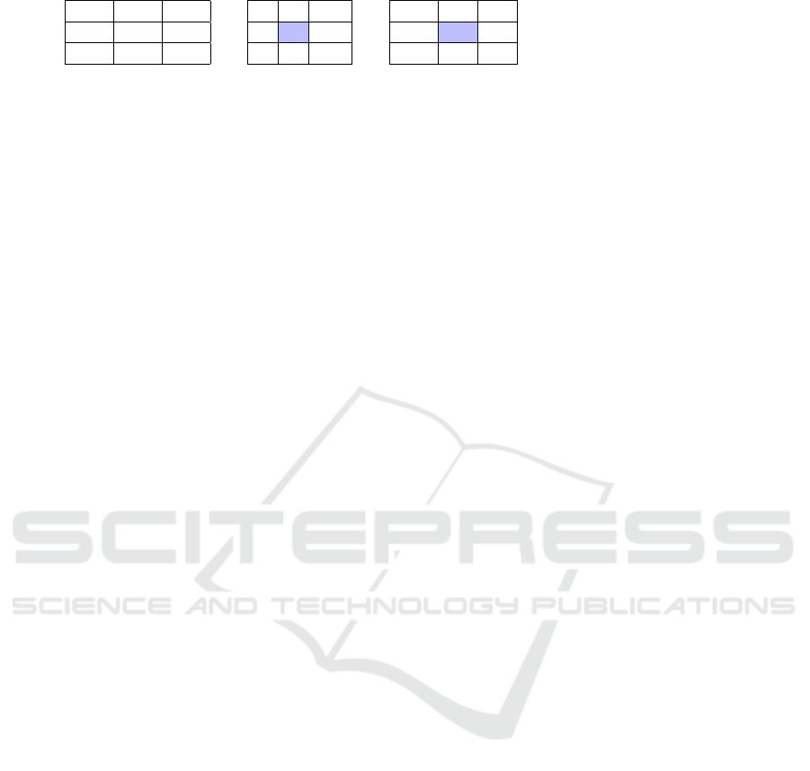
Example 3 (Application of ROI to Textured Image).

Consider now the neighborhood of a pixel ’p’ in a

image I, i.e. the set of pixels that touch it. The neigh-

borhood of a pixel can have a maximum of 8 pixels as

shown in Fig. 3a. The colored pixels in Fig. 3b are

8-connected to p.

For instance, the 4 ×4 image I in Fig. 3a. can be

decomposed using the 8-connectivity into the 16×8

matrix R = {r

,. .. ,r

} (Fig. 3b where r

denotes

the column of pixel 1 (clock-wise ordering), r

de-

notes the column of pixel 2, and so on. The same

principle as for LBP is mimic, but with the transfor-

mation given in Eq. (15). The 8 neighbors around the

central pixel can be seen as ”voters” from whom we

expect a total rank-order.

The 8-connectivity matrix R is transformed into

ranks by simple ordering on which we can apply algo-

rithm 1. Concerning on peripheral pixels, the spatial

area is enlarged by adding borders of zeros. In gen-

eral, if our image is of size n ×n, and we examine a

neighborhood of f × f , then the size of the resulting

output is (n − f +1)×(n − f +1). With n = 4, f = 3,

indeed, this gives us a 2 ×2 output channel. For a

n ×n image, the encoding values are between 1 and

. The generalization to larger images is straightfor-

ward.

a question that might arise is how to choose the

ranks for the tied values? it was shown in (Vigneron

The Kendall’s coefﬁcient is a statistic used to measure

the ordinal association between two measured quantities.

As the correlation coefﬁcient value goes towards 0, the re-

lationship between the two variables will be weaker.

LBP weights

1 2 3

8 4

7 6 5

(a) Neighbor pix-

els ordering.

(b) The orange pixels form the neighborhood of the

pixel ’p’.

Figure 3.

1 2 3 4

1 4 8 20 18

2 17 12 17 17

3 6 1 17 17

4 4 6 5 14

(a) 4 ×4 image I.

center

pixel

12 4 8 20 17 17 1 6 17

17 8 20 18 17 17 17 1 6

1 17 12 17 17 5 6 4 6

17 12 17 17 17 14 5 6 1

(b) 8-connectivity matrix R.

center

pixel

12 1 1 4 1 4 1 3 4

17 1 4 3 2 3 4 1 3

1 4 2 2 3 1 3 2 2

17 3 3 1 4 2 2 4 1

Figure 4.

and Tomazeli Duarte, 2018) that the encoding is in-

sensitive to ties.

As an illustration LBP is applied to Lena’s origi-

nal picture 5a and provides the texture representation

given in Figure 5b. From the ﬁgure 5a, we obtained a

ICINCO 2022 - 19th International Conference on Informatics in Control, Automation and Robotics

590

new decomposition (Figures 5c-5f). Visually, the 1st

plot is more informative than the 2nd one, which itself

is nore informative than the 3rd, and so on.

(a) Original (b) Classic LBP

(e) ROI comp. 3 (f) ROI comp. 8

Figure 5: Lena’ original (a) is compared to classic LBP rep-

resentation (b) and with the 1st, 2nd, 3rd and eighth rank-

order components obtained from Algorithm 1. The eighth

component is apparently the less informative component.

5 ROI-pooling OPERATOR

In CNNs maximum pooling operator is deﬁned

mathematically for a volume V : A → R, A =

{(i

,. .. ,i

)|i

∈ [1,...,n

],k ∈ [1, .. ., N]} and a

set B = {(i

,. .. ,i

N−1

,0)|i

∈ [−K

,. .. ,K

],b ∈

[1,. .. ,N −1]} called window where either K

= K

or K

= K

−1 with K

∈ N as follows:

maxpool = max

y∈B

f (x −y). (17)

The operation in Eq. 17 looks for the maximum in a

neighborhood given by B along the image axis. Un-

like the convolution operator, the pixel values in this

neighborhood are not combined. Often the maximum

pooling operation is used for downsampling the vol-

ume by restricting x (striding) with stride s ∈ N and A

is restricted to A

′

= {(i

,. .. ,i

)|i

∈ [1,1 + s,1 +

2s,. .. ,1 +n

s],n

= ⌈n

/s⌉−1,k ∈ [1 ...N]} with the

ceiling function ⌈·⌉. The strided maximum pooling

operation is then:

′

= 1 + sx, max pool = max

y∈B

f (x

′

−y) (18)

where B is simply a binary mask. The strided max-

imum pooling reduces the size of the input image

by only considering every s−th entry along all im-

age axes and discarding all others. ROI-pooling can

easily replace maximum polling in CNN:

ROI pooling( f ,B) = ROI f (x

). (19)

In Eq. 19, y is put for the neighborhood in which

x is selected. As maximum pooling, ROI pooling is

parameter free.

To answer to the question if could ROI pool-

ing perform as well as max-pooling in 19, different

grouping operations were performed in a categoriza-

tion context.

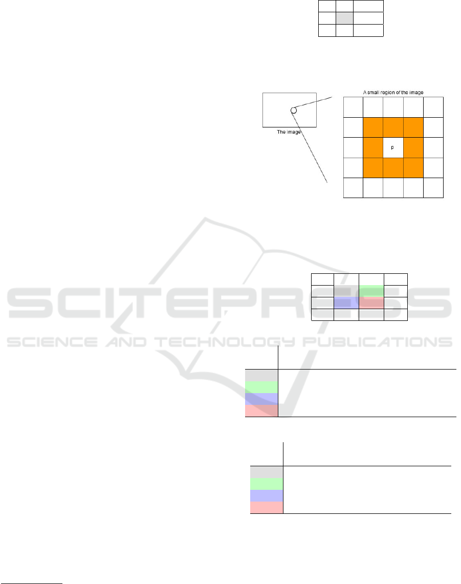
Example 4 (ROI Pooling for Automatic Lesion

Segmentation of Stroke Patient). Lack of expertise

or time for interpreting a brain magnetic resonance

imaging (MRI) in the case of stroke increases the risk

of death and disability. This study aims to enable

rapid and accurate assessment of the damage caused

by hyperacute ischemic stroke (< 4.5h) by quantifying

the volume of ischemia. By reducing the variability of

interpretation, it enables a more standardized stroke

diagnosis, and facilitates rapid and consistent treat-

ment decisions by health professionals regardless of

their experience or expertise.

MRI provides information about damage to the

brain. Combined with medical knowledge on blood

ﬂow in the human brain, MRI makes it possible to

identify the thrombus causing the problems and to de-

cide on the treatment of endovascular recanalization

(single or double thrombolysis, thrombectomy).

The stroke dataset was provided with the support

of the neurology group of the Center Hospitalier Sud

Francilien (see (Kobold et al., 2019) for a full descrip-

tion of the dataset). It contains the cranial MRI of 65

stroke patients. The MRI modalities available for this

data set are DWI B0 ADC FLAIR ToF and the corre-

sponding phase modalities. 61 of the patients show a

lesion on DWI, but some exams lack the phase image.

Thus there are only 58 patients with a visible le-

sion on DWI where all terms are available. The 65

Importance Order Ranking for Texture Extraction: A More Efﬁcient Pooling Operator Than Max Pooling?

591

(a) Maximum intensity projection of a patient with mid-

dle carotid artery (MCA) occlusion.

(b) Intensity of injury comparable to that of normal tis-

sue.

Figure 6: Development of a lesion visualized on diffusion

imaging (DWI). (a) The artery stops abruptly at the point

of occlusion (1) (b) Most of the publications deal only with

well developed lesions which take advantage of the high

intensity boundaries. In the hyperacute phase, these borders

are weak or zero and weak intensities complicate the task of

segmentation.

patients all have a visible lesion. MRIs were acquired

from a 1.5 T and 3 T General Electrics MRI machine.

DWI B0 and ADC share the same resolution, as they

are from the same acquisition.

Manual lesion segmentations are available. All

lesions were segmented by at least two neurolo-

gists. Inter-observer agreement, measured in terms of

Dice’s coefﬁcient, was 0.69 ±0.15. The median le-

sion size in the data set is approximately 2,920 voxels:

the MRI is taken in the hyperacute phase of the stroke,

which means that the lesion is growing, may be small

and does not have a well-deﬁned border. This makes

it a more difﬁcult task than the cases that have already

been studied in the literature.

Data augmentation is used because the training set

is too small to generate a model that generalizes well.

Random crops linked to plot sampling works as fol-

lows: the plots are sampled at a size larger than the

intended size for training. For example, the model

is trained on 64×64 then the patches are sampled at

74×74. Then, during training, a 64×64 image is cut

from the 74×74 patch in a random location, but in

such a way that the 64×64 image is entirely contained

in the 74×74 image. The number of possible random

crops for a patch is determined by the patch size dif-

ference and the size of the training image. Once data

is co-registered and normalized, automatic lesion seg-

mentation is performed.

The most common evaluation metric for evaluat-

ing biomedical image segmentations is Dice’s coef-

ﬁcient which measures the overlap of two segmen-

tations but also takes into account their cardinality.

This dependence on cardinality makes it difﬁcult to

tell which value of Dice’s coefﬁcient indicates a good

segmentation result. A perfect segmentation is iden-

tical to the ground truth and gives a Dice’s coefﬁcient

of 1. If there is no overlap, then the dice is 0.

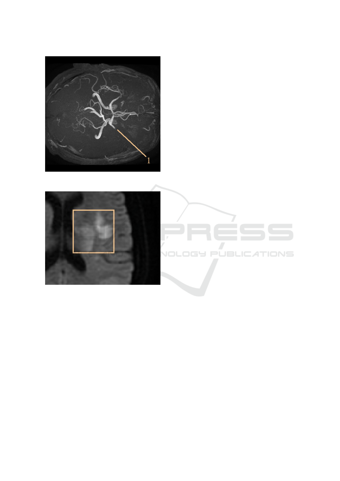
The ﬁrst method tried is 2d U-Net, trained on

64×64 patches using enhanced lesion image with

DWI (see Fig. 7). 3d U-net, CNN and improved U-

net with ROI were tested.

The segmentation results of the four networks are

given in the table 4. The 3D U-Net again suffers from

the small training set whereas the U-Net generally

learns to detect the lesion but fails in some cases.

The fewer false positive number is found with U-

Net with Spearman ROI. Upon manual inspection,

it turns out that these are very close to the main le-

sion and may even be part of the lesion, depending on

the deﬁnition. It is therefore an almost perfect result.

Since the false positives were an insigniﬁcant amount

of voxels anyway, the Dice coefﬁcient only changes at

the fourth digit after the decimal indicate. This result

is therefore a segmentation of the lesion at the human

level. It is in particular the ﬁrst lesion segmentation

that achieves this performance and a better result can-

not be achieved on this type of database. Figure 7

shows an instance of gradual contours of the develop-

ing lesion and contralateral artifacts that only trained

experts can identify as such.

ICINCO 2022 - 19th International Conference on Informatics in Control, Automation and Robotics

592

Table 4: Segmentation results for the thrombus. The columns are the Dice coefﬁcient, the mean number of false positive

objects FP and the average ”FP Size”, the mean number of false negative objects FN and their average size ”FN Size” and

the detection rate Dr.

Model Dice FP FP Size FN FN Size Dr

U-Net 0.65 3.3 29.6 0.39 239.5 0.93

3D U-Net 0.56 229.7 215 1.48 643.5 1.0

CNN 0.53 208.3 83.8 0.25 263.9 0.89

U-Net+Spearman ROI 0.8 133.6 94.0 0.14 353.8 0.96

U-Net+ absolute rank ROI 0.76 29.8 76.3 0.25 121.1 1.0

Figure 7: An example of lesion development in the hyperacute phase of stroke (left). The lesion is currently growing and has

no clearly deﬁned borders but instead shows gradients towards normal tissue. The image in the center shows the ground truth

and the one on the right the probability of injury given by the model. Please note that our algorithm correctly identiﬁed the

contralateral artifact.

6 CONCLUSION

The rank-order pooling layers are non parametric, in-

dependent of the geometric arrangement or sizes of

the image regions, and can therefore better tolerate

rotations. An other asset of the rank-order pooling

lies in the number of rank-order components g

ℓ

that

the algorithm 1 can generate, which are uncorrelated

from each other and which guarantees optimal (inde-

pendent) feature extraction performance.

When should we pool and when should we not?

The answer depends upon the following considera-

tions, in descending order of importance: (i) if there is

an inadequate number of observations in each of two

(or more) subgroups, which would usually necessitate

pooling (ii) common sense, necessity, etc.

In statistics, ”pooling” means gathering together

small sets of data that are assumed to have the same

value of a characteristic. ROI pooling is transform-

ing convolution features into a new representation that

preserves important information while ignoring irrel-

evant details.

REFERENCES

Benson, D. (2016). Representations of Elementary Abelian

p-Groups and Vector Bundles. Cambridge tracts in

mathematics. Cambridge University Press, 1 edition.

uggemann, R. and Patil, G. (2011). Ranking and Prior-

itization for Multi-indicator Systems: Introduction to

Partial Order Applications. Environmental and Eco-

logical Statistics. Springer-Verlag New York.

Diaconis, P. (1988). Group Representation in Probability

and Statistics., volume 11 of IMS Lecture Series. In-

stitute of Mathematical Statistics, Harvard, USA.

Gehrlein, W. and Lepelley, D. (2011). Voting Paradoxes and

Group Coherence: The Condorcet Efﬁciency of Voting

Rules. Studies in Choice and Welfare. Springer-Verlag

Berlin Heidelberg, 1 edition.

Goodfellow, I., Bengio, Y., and Courville, A. (2016). Deep

learning, volume 1. MIT press Cambridge.

Haralick, R. (1979). Statistical and structural approaches to

texture. In Proceedings of the IEEE, volume 67, pages

786–804.

Kobold, J., V., V., Maaref, H., Fourer, D., Aghasaryan, M.,

Alecu, C., Chausson, N., L’hermitte, Y., Smadja, D.,

and L

ang, E. (2019). Stroke Thrombus Segmenta-

tion on SWAN with Multi-Directional U-Nets. In 9th

IEEE International Conference on Image Processing

Theory, Tools and Applications (IPTA 2019), Proc. of

Importance Order Ranking for Texture Extraction: A More Efﬁcient Pooling Operator Than Max Pooling?

593

the 9th IEEE International Conference on Image Pro-

cessing Theory, Tools and Applications (IPTA 2019),

Istanbul, Turkey.

Lazebnik, S., Schmid, C., and Ponce, J. (2006). Beyond

bags of features: Spatial pyramid matching for rec-

ognizing natural scene categories. In Proceedings of

IEEE Computer Society Conference on Computer Vi-

sion and Pattern Recognition, volume 2, pages 2169 –

2178.

Ojala, T., Pietik

ainen, M., and Harwood, D. (1996). A com-

parative study of texture measures with classiﬁcation

based on feature distributions. Pattern Recognition,

29:51–59.

Pietikinen, M., Hadid, A., Zhao, G., and Ahonen, T. (2011).

Computer Vision Using Local Binary Patterns, vol-

ume 40 of Computer imaging and vision. Springer.

Savage, R. (1956). Contributions to the theory of rank-order

statistics – the trend case. The Annals of Mathematical

Statistics, 27(3):590–615.

Tan, X. and Triggs, B. (2007). Enhanced local texture fea-

ture sets for face recognition under difﬁcult lighting

conditions. In Analysis and Modeling of Faces and

Gestures, volume 4778 of Lecture Notes in Computer

Science, pages 235–249, Berlin. Springer.

Vigneron, V. and Duarte, L. (2017). Toward rank disag-

gregation: An approach based on linear programming

and latent variable analysis. In Tichavsk

y, P., Babaie-

Zadeh, M., Michel, O. J., and Thirion-Moreau, N., ed-

itors, Latent Variable Analysis and Signal Separation,

pages 192–200, Cham. Springer International Pub-

lishing.

Vigneron, V. and Petit, E. (2008). The evaluation of the

impact of the technology transfers from public labora-

tories to private ﬁrms : the case of the french nuclear

authority. Fuzzy Economic Review, 13(1).

Vigneron, V. and Tomazeli Duarte, L. (2018). Rank-order

principal components. A separation algorithm for or-

dinal data exploration. In 2018 International Joint

Conference on Neural Networks, IJCNN 2018, Rio de

Janeiro, Brazil, July 8-13, 2018, pages 1–6.

Yadav, N.. author. abd Yadav, A. and Kumar, M. (2015). An

Introduction to Neural Network Methods for Differen-

tial Equations. Springer, Gurgaon, Haryana, India.

Yu, D., Wang, H., Chen, P., and Wei, Z. (2014). Mixed

pooling for convolutional neural networks. In Inter-

national Conference on Rough Sets and Knowledge

Technology, pages 364–375.

ICINCO 2022 - 19th International Conference on Informatics in Control, Automation and Robotics

594