A Faster Converging Negative Sampling for the Graph Embedding

Process in Community Detection and Link Prediction Tasks

Kostas Loumponias

, Andreas Kosmatopoulos

, Theodora Tsikrika

, Stefanos Vrochidis

and Ioannis Kompatsiaris

Information Technologies Institute, Centre for Research and Technology Hellas - CERTH, GR-54124, Thessaloniki, Greece

Keywords:

Skipgram Algorithm, Negative Sampling, Graph Embedding, Community Detection, Link Prediction.

Abstract:

The graph embedding process aims to transform nodes and edges into a low dimensional vector space, while

preserving the graph structure and topological properties. Random walk based methods are used to capture

structural relationships between nodes, by performing truncated random walks. Afterwards, the SkipGram

model with the negative sampling approach, is used to calculate the embedded nodes. In this paper, the

proposed SkipGram model converges in fewer iterations than the standard one. Furthermore, the community

detection and link prediction task is enhanced by the proposed method.

1 INTRODUCTION

Neural network applications have expanded signiﬁ-

cantly in recent years in various scientiﬁc ﬁelds, such

as image classiﬁcation (He et al., 2019), natural lan-

guage processing (Chowdhary, 2020), and network

analysis (Nguyen et al., 2018). A particularly suc-

cessful utility of deep learning is the embedding pro-

cess (Cai et al., 2018), which is used for mapping dis-

crete variables to continuous vectors. This technique

has found practical applications in graph embedding,

enabling the use of such methods for network anal-

ysis tasks, such as community detection (Rozember-

czki et al., 2019; Cavallari et al., 2017) and link pre-

diction (Grover and Leskovec, 2016).

Graph embedding is an approach that is utilised

to transform nodes, edges, and their features into a

lower dimensional vector space, while the properties,

like the graph structure and topological information,

are preserved. Graph embedding is a complex pro-

cess, since the graphs may vary in terms of their scale

and speciﬁcity. Therefore, a variety of approaches

for embedded graphs have been proposed (Goyal and

Ferrara, 2018), each with a different level of granular-

ity. In particular, the embedding methods can be cat-

https://orcid.org/0000-0002-6268-3893

https://orcid.org/0000-0001-5334-741X

https://orcid.org/0000-0003-4148-9028

https://orcid.org/0000-0002-2505-9178

https://orcid.org/0000-0001-6447-9020

egorised as follows: (a) factorization based, (b) deep

learning based, and (c) random walk based.

Factorization based algorithms aim to factorize

the matrix that represents the connections between

the nodes of the graphs, in order to obtain the em-

bedding. In the case where the obtained matrix is

positive semideﬁnite, such as the Laplacian matrix,

the eigenvalue decomposition can be utilized. Deep

learning-based algorithms attempt to preserve the ﬁrst

and second order network proximities by using deep

autoencoders, due to their ability to model non-linear

structure in the data. Random walk based algo-

rithms are used to capture structural relationships be-

tween nodes, by performing truncated random walks.

Therefore, a graph is transformed into a collection of

node sequences, in which, the occurrence frequency

of a vertex-context pair measures the structural dis-

tance between them (Zhang et al., 2018). Some of

the most popular random walk based methods are

DeepWalk (DW) (Perozzi et al., 2014) and node2vec

(n2v) (Grover and Leskovec, 2016).

DW aims to learn embedded nodes via a ran-

dom walk sampling process and the word2vec algo-

rithm (Mikolov et al., 2013a). In word2vec, the Skip-

Gram model is applied by using sentences (series of

words) to train the embedded word. In a nutshell, the

training objective is to use the center word in order to

predict surrounding words of the sentence. Hence, the

DW process initially starts from an arbitrary node and

performs transitions to neighboring nodes in an uni-

form fashion (i.e. all neighbors of a node have equal

Loumponias, K., Kosmatopoulos, A., Tsikrika, T., Vrochidis, S. and Kompatsiaris, I.

A Faster Converging Negative Sampling for the Graph Embedding Process in Community Detection and Link Prediction Tasks.

DOI: 10.5220/0011142000003277

In Proceedings of the 3rd International Conference on Deep Learning Theory and Applications (DeLTA 2022), pages 86-93

ISBN: 978-989-758-584-5; ISSN: 2184-9277

probability of being selected). A walk process is ter-

minated upon reaching a maximum length which is

predeﬁned (user-provided parameter). This process is

applied for all nodes and is repeated n times (number

of walks). It follows that a node and a series of nodes

can be treated as a word and a sentence, respectively,

enabling, the SkipGram algorithm to be naturally uti-

lized for generating node embeddings.

One of the disadvantages of DW is that it cannot

control the path generated by the random walk. In or-

der to address this limitation, the n2v approach has

been proposed. In particular, n2v uses random walks

(similarly to DW) with transition probabilities that are

governed by weights, i.e., n2v generates biased walks.

Instead of performing walking steps randomly, the

concepts of Breadth-First-Search (BFS) and Depth-

First-Search (DFS) sampling are introduced to control

random behavior.

An important characteristic of the original Skip-

Gram implementation is that it’s based in the use of

the softmax function which can result in a very ex-

pensive computational cost. To alleviate this problem

the negative sampling process is utilised which oper-

ates under a lower computational complexity cost and

typically offers better execution times. The negative

sampling process uses the sigmoid function to differ-

entiate the actual context nodes (positive) from ran-

domly drawn nodes (negative). The negative samples

are selected via the noise distribution (Mikolov et al.,

2013b). However, the main drawback of the sigmoid

function is the vanishing gradient problem (Hochre-

iter, 1998) which ultimately leads to a slower conver-

gence of the SkipGram model.

In this paper, a modiﬁed SkipGram algorithm

is proposed for the DW and n2v processes to

achieve faster convergence in community detection

and link prediction tasks compared to the standard

DW and n2v processes, preserving the accuracy in

both tasks.More speciﬁcally, a novel function, σ

(x),

with an additional trainable parameter is proposed to

tackle the limitations of a standard sigmoid function.

In addition, the new gradients in the backward propa-

gation process are calculated and explained in detail.

Finally, the calculated embedded nodes are used in

the community and link prediction task. More specif-

ically, and after producing the graph embeddings, the

k-means algorithm (Hartigan and Wong, 1979) is ex-

ecuted to obtain the ﬁnal communities, while the lo-

gistic regression model (Hosmer Jr et al., 2013) with

the consideration of various similarity measures is

utilised to predict the existence of links between two

nodes in the graph. The experimental results in real

graphs show that the proposed method converges (i.e.

the k-means algorithm and logistic regression model

Input Layer Hidden Layer Output Layer

𝑾

𝒚

𝑘−𝑤

𝑾

𝒖

𝑘

𝒛

𝑘

𝑉 𝑥 𝑑 𝑑 𝑥 𝑉

𝑾

𝒚

𝑘+𝑤

One-hot vector d-dim

Figure 1: The SkipGram model.

achieve their optimal results) faster and provides more

coherent community detection and link predictions

results than the standard DW and n2v processes.

2 PROPOSED METHOD

A general overview and mathematical formulation of

the SkipGram algorithm under the negative sampling

approach is provided. Following that, the proposed

DW (and n2v) algorithm using a modiﬁed SkipGram

model is described.

2.1 SkipGram Model: The Negative

Sampling Approach

Let G = (V, E) be a graph, where V and E ⊆ (V ×V )

correspond to the node and edge set of the graph, re-

spectively. Figure 1 illustrates the SkipGram model

where it can be seen that it corresponds to a fully

connected neural network with one hidden layer and

multiple outputs. The SkipGram model attempts to

predict the context nodes of a sentence (a series of

nodes) given the target node. The input vector u

the one-hot embedded vector of target node u

∈ V ,

∈ M

|V |×d

is the embedding matrix, where

de-

notes the total number of the nodes and d the embed-

ding size. Each row of W

represents the embedded

vector of node u

∈ V . The vector z

∈ R

stands for

the embedded vector of node u

and is equal with

= W

· u

. (1)

∈ M

d×|V |

is the output embedding matrix, while

k−w

, ..., y

k−1

, y

k+1

, ..., y

k+w

} are the predicted con-

text nodes (one-hot vectors) when the input-target

node is u

, where w denotes the window size.

In the vanilla SkipGram model, the cost function

J is calculated via the softmax function as

J(θ) = −

∑

c=1

log

exp



· z



∑

|V |

i=1

exp



· z



, (2)

A Faster Converging Negative Sampling for the Graph Embedding Process in Community Detection and Link Prediction Tasks

where θ = [W

, W

] and W

stands for the i-th col-

umn of the output embedding matrix W

and C de-

notes the total number of context nodes. Furthermore,

the term

P(u

;θ) =

exp



· z



∑

|V |

i=1

exp



· z



(3)

represents the conditional probability of observing a

context node u

given the target node u

From (2), it follows that the softmax function is

computationally expensive, as it requires scanning

through the entire output embedding matrix W

compute the probability distribution of all nodes ∈ V .

Furthermore, the normalization factor in the denom-

inator (2) also requires

iterations. Due to this

computational inefﬁciency, softmax function is not

utilised in most implementations of SkipGram.

Thereafter, the negative sampling process with

sigmoid function is used, which reduces the complex-

ity of the algorithm. More speciﬁcally, for each posi-

tive pair, {u

and u

} in the training sample, K number

of negative samples are drawn from the noise distribu-

tion P

(w) (Mikolov et al., 2013b), and the model will

update (K + 1) × d neurons in the matrix W

, where

K is usually set equal to 5. Thus, the logarithm of the

conditional probability (3) is approximated by

logP(u

;θ) = log σ



· z



∑

i=1

logσ



−W

neg(i)

· z



, (4)

where σ(x) is the sigmoid function, while

neg(i)

}

i=1

is the set of columns W

(vectors

d × 1) which are randomly selected from the noise

distribution P

(w). The ﬁrst term of (4) indicates

the logarithmic probability of the positive sample u

to appear within the context window of the target

node u

, while, the second term indicates the sum of

the logarithmic probabilities of the negative samples

neg(i)

not appearing in the context window.

In the negative sampling process, only K + 1

columns of the output embedding matrix W

are up-

dated, while in the embedding matrix W

only one

row is updated (let W

∈ R

), since the input u

one-hot vector. Then, the update equations, through

the backward propagation, are

= c

− η · (σ(x

) −t

) · z

, (5)

= W

− η ·

K+1

∑

j=1

(σ(x

) −t

) · c

, (6)

where

(

, j = 1

neg( j−1)

, j = 2, ..., K + 1

(

1, j = 1

0, j = 2, ..., K + 1

= c

· z

and η is the learning rate.

In the case where j = 1 (positive sample) and x

→

−∞, the term −(σ(x

) −t

) is maximized. Therefore,

the SkipGram model updates-corrects the weights θ =

, W

] for low values of x

, otherwise, when the

values of x

are high, the updates, − (σ(x

) −t

) are

negligible. In the same way, for j 6= 1 (negative sam-

ples), it turns out that for low values of x

, the updates

are negligible. Thus, the inner product x

= c

· z

de-

ﬁnes a proximity between the nodes u

and u

2.2 SkipGram with a Modiﬁed Negative

Sampling Process

The main drawbacks of the sigmoid function are the

vanishing gradient of log σ(x) (O log σ(x)) and its sat-

urated values. More speciﬁcally, as it can be seen

in Figure 2, the gradient O log σ(x) (blue curve) con-

verges to 0 for x → +∞ and to 1 for x → −∞. Thus,

in the case where j = 1 (positive sample) for every

low value of x

the gradient is approximately equal to

1. Hence, the range of the updates is limited and the

highest value that it can reach is equal to 1. This can

cause a lot of computational burden until the weights

θ converge.

In order to overcome the above limitation, the sig-

moid b function is proposed

(x) =

1 + exp(−b · x)

, (7)

where b > 1. It is worth noting that the range of the

proposed function is the interval [0, 1], since it ap-

proximates the probability (4). In Figure 2, the deriva-

tive of logσ

(x) (9) for b = 2 is illustrated. As it can

be seen the range of the proposed derivatives is [0,2].

The logarithm of the conditional probability (3) in

the proposed method is equal to

logP(u

;θ) = log σ



· z



∑

i=1

logσ



−W

neg(i)

· z



. (8)

-10 -5 0 5 10

0.5

1.5

b=2

(x)

Figure 2: The derivatives of log σ(x) and log σ

b=2

(x).

DeLTA 2022 - 3rd International Conference on Deep Learning Theory and Applications

Then, it is proved that the derivative of log σ

(x) is

equal with

O log σ

(x) =

∂σ

(x)

∂x

= b · (1 − σ

(x)). (9)

Thus, using (8) and (9) the update equations for the

proposed SkipGram model (SkipGram

) are deﬁned

= c

− η · b ·(σ

) −t

) · z

, (10)

= W

− η · b ·

K+1

∑

j=1

(σ

) −t

) · c

. (11)

It is important to note that, in the proposed process,

the additional parameter b is trainable and the update

equation (using (8) and (9)) is proved to be equal with

b = b − η

K+1

∑

j=1

(σ

) −t

) · x

, (12)

where η

is the learning rate for the parameter b.

From (12), it can be straightforwardly deduced that

the updates of parameter b will be negligible when the

error (σ

) − t

) is reduced. It is derived from the

above results that the proposed sigma function can be

applied to any machine learning model instead of the

standard sigma function, however the updates equa-

tions (10)-(12) need to customized to the applicable

machine learning model.

It is worth mentioning that in literature there have

been alternative activation functions proposed aiming

for better performance in various scientiﬁc ﬁelds. In

(Banerjee. et al., 2021), the SM-Taylor softmax func-

tion has been applied for image classiﬁcation tasks

and the results showed that it outperforms the normal

softmax function.

Next, the proposed process (Algorithm 1) for

community detection is presented. The proposed

method, DeepWalk

(DW

) has similar framework to

DW, with the main difference being the use of the

SkipGram

model instead of the standard one. In the

following, lines 1 − 7 in (Algorithm 1) represent the

process. Then, the k−means algorithm is used

to detect the communities of the graph (Com). As

a ﬁnal remark, we note that the proposed SkipGram

model can be also applied to the n2v process, since the

only difference between DW and n2v is the way that

random walks are performed (line 4 of Algorithm 1).

In Algorithm 2 the process of link prediction as

well as the evaluation process is presented. More

speciﬁcally, three sub-graphs G

, G

mod

and G

are

derived from the initial graph G. Initially, the train

graph G

is used to calculate the embedded nodes

. Then, the similarities between embedded nodes

are calculated using various operators (oprtr), such as

Hadamard product, L1, L2 norm (Luo et al., 2016)

etc., afterwards the logistic regression model is used

to calculate the classiﬁers (whether the nodes are con-

nected or not). Next, the classiﬁers (one for each op-

erator) are evaluated considering the model selection

graph G

mod

and the embeddings θ

. Finally, the op-

erator with the highest accuracy score is utilised to

evaluate the classiﬁer for the test graph G

Algorithm 1: DeepWalk

for community detection.

Require: Graph G, number of communities k, window size

w, embedding size d, walk length t, number of walks n

1: for i=1:n do

2: O = Shu f f le(V )

3: for u

∈ O do

4: RW

= RandomWalk(G, u

,t)

5: θ = SkipGram

(RW

, w)

6: end for

7: end for

8: Com = k-means(θ,k)

9: return Com

Algorithm 2: DeepWalk

for link prediction.

Require: Graph G, window size w, embedding size d, walk

length t, number of walks n

1: G

, G

mod

, G

= split(G)

2: θ

= DW

, w, d, t, n)

3: for i=1:ν

oprtr

4: clsfr(i) = Logistic Regression(θ

, operator(i))

5: AccScore(i) = evaluate(clsfr(i), G

mod

, θ

, oprtr(i))

6: end for

7: i

max

= argmax(AccScore)

8: cls f r

max

, oprtr

max

= clsfr(i

max

), oprtr(i

max

)

9: θ

= DW

tsr

, w, d, t, n)

10: Test Score = evaluate(cls f r

max

, G

, θ

, oprtr

max

)

3 EXPERIMENTAL EVALUATION

In this section, we conduct experimental evaluation

on the proposed methods, DW

and n2v

(n2v using

SkipGram

algorithm) against the standard DW and

n2v process, respectively. To that end, real datasets

with ground-truth communities are used. We use

publicly available graphs Cora, Pubmed and Cite-

Seer (Sen et al., 2008) for evaluation, which are

provided with ground-truth communities. The Cora

dataset consists of 2708 publications, classiﬁed into 7

classes, and 5429 links. The PubMed dataset consists

of 19717 publications, classiﬁed into 3 classes, and

44338 links. The CiteSeer consists of 3312 publica-

tions, classiﬁed into 6 classes, and 4732 links.

The parameters used in methods DW

, n2v

, DW

and n2v are w = 10 (window size), d = 128 (embed-

ding size), t = 80 (walk-length) whereas the number

of epochs and the batch-size are equal to 10 and 1000,

A Faster Converging Negative Sampling for the Graph Embedding Process in Community Detection and Link Prediction Tasks

respectively. Parameters p and q used in n2v

and n2v

were evaluated using a grid search over [0.25, 0.5, 1,

2, 4] (Grover and Leskovec, 2016). The experimen-

tal sets are conducted considering different values of

learning rate, η ∈ {0.05, 0.2,0.6, 1.0, 2.0}. Further-

more, in the proposed processes, the learning rate of

the parameter b is set equal to η

= 0.01 for all exper-

imental sets. This value is often considered as a typi-

cal value for the learning rate, while our experiments

with η

values close to it provided a stable training

in the experimental sets; in future work, further val-

ues of η

will also be considered. Finally, all meth-

ods use the stochastic gradient descent technique with

momentum 0.9 for the back propagation process.

Regarding the community detection task, in each

experiment, the Adjusted Rand Index (ARI), the Nor-

malized Mutual Information (NMI) and the graph’s

modularity (Mod) (Vinh et al., 2010) are calculated,

while, for the link prediction task the Area Under

the Curve (AUC) score (Fawcett, 2006) is calcu-

lated. Furthermore, the StellarGraph tool (Grover

and Leskovec, 2016) is used to split the input graph

G = (V,E) to G

= (V,E

), G

mod

= (V,E

mod

) and

= (V, E

). In all datasets, E

includes 90% of the

total edges (E), while the E

and E

mod

include 75%

and 25% of E

, respectively.

3.1 Evaluation of the Modiﬁed

DeepWalk and Node2vec

In this section, the performance of the DW, DW

n2v and n2v

methods is presented. Figure 4 illus-

trates the performance of DW and DW

considering

the metrics ARI, NMI, Mod and AUC (y axis) for dif-

ferent values of η in the CiteSeer, Cora and PubMed

graph. Moreover, the x axis in the sub-ﬁgures stands

for the number of epochs. It is clear, that the pro-

posed method, DW

, converges faster than the stan-

dard one, DW, in all datasets for all the different val-

ues of η. Additionally, it can be observed that the

DW process for η = 0.05, does not converge within

10 epochs (i.e more than 10 epochs are required) in

any of the datasets.

In case of a lower value of η, the convergence

speed will be further reduced, therefore, lower learn-

ing rates are not considered in this paper. As an ex-

ample, a learning rate equal to 0.005 is used for the

CiteSeer graph to verify the above statement. Figure

3 illustrates the loss values of DW and DW

in the

community detection task for each epoch. It is clear

that the DW process is not able to converge within

100 epochs, while DW

can converge to 30 epochs,

due to the trainable parameter b.

More details about the convergence speed in com-

0 10 20 30 40 50 60 70 80 90 100

Epochs

0.5

1.5

2.5

3.5

4.5

Loss

DW Loss

Loss

Figure 3: The loss values of DW and DW

in community

detection task, for the CiteSeer graph with η = 0.005.

munity detection and link prediction task for DW

and DW

are provided in Table 1. The columns cd

epochs and lp epochs stand for the required number

of epochs in order for the community detection met-

rics (i.e. ARI, NMI, Mod) and link prediction metric

(AUC) to converge. It is demonstrated that the DW

process outperforms the standard DW, considering the

convergence speed (in both tasks) in all experimental

sets apart from one. More speciﬁcally, only in the

PubMed graph for η = 2.0, the two methods require

the same number of epochs. Moreover, it is worth not-

ing that DW

is more robust in terms of converging

speed at different values of η than the standard DW,

since DW

uses the introduced trainable parameter b.

In addition, the proposed method provides the

same (or better) performance as DW in the com-

munity detection and link prediction tasks in fewer

epochs. In Table 1, the best performances of all met-

rics, within 10 epochs, for both methods are provided.

As it can be seen, the best performances of the met-

rics, regardless of the learning rate, are similar (the

differences are less than 10

−2

) for both methods in

most experiments. However, in the CiteSeer graph,

has ARI score equal to 0.1409 (η = 2.0), while

the highest ARI score for DW is equal to 0.1235

(η = 2.0). In addition, the highest Mod and AUC

score for DW

are equal to 0.7358 (η = 1.0) and

0.9207 (η = 0.6), respectively, while the highest val-

ues of DW are equal to 0.7224 (η = 2.0) and 0.9105

(η = 2.0). Finally, in Pubmed graph, DW

has AUC

score equal to 0.8674 (η = 0.6), while the highest

AUC score for DW is equal to 0.7779 (η = 2.0).

The performances of n2v and n2v

in the commu-

nity detection and link prediction tasks are provided

in Table 2 and Figure 5, in a similar way as in Table 1

and Figure 4, respectively. It can be observed that the

n2v

process outperforms the standard n2v process,

considering the convergence speed (in both tasks), in

all experimental sets, apart from the PubMed graph

for η = 2, where both n2v and n2v

require 1 epoch

to converge. As it can be seen in Table 2, n2v

pro-

vides a more robust converging speed (for both tasks)

at different values of η than the standard n2v.

DeLTA 2022 - 3rd International Conference on Deep Learning Theory and Applications

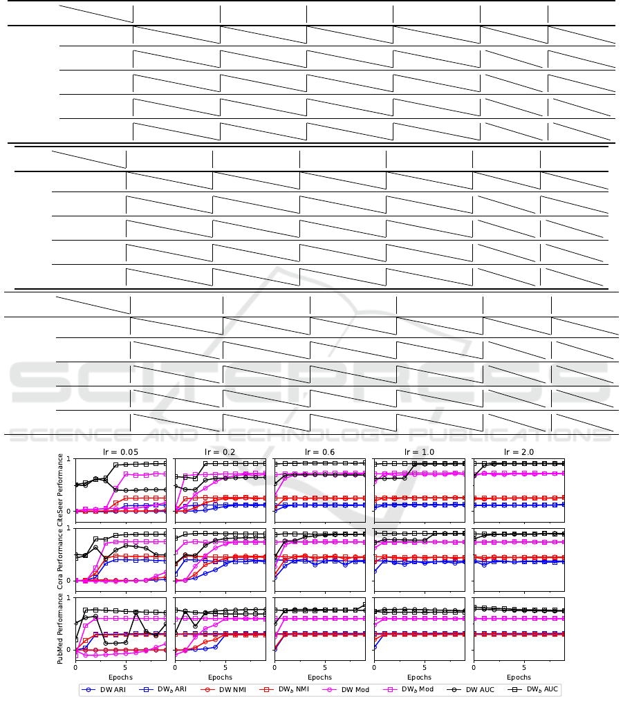
Table 1: The best performances of DW and DW

regarding the metrics ARI, NMI, Mod and AUC. The columns cd epochs

and lp epochs contain the required number of epochs in order for the community detection metrics (i.e. ARI, NMI, Mod) and

link prediction metric (AUC) to converge.

ARI NMI Mod AUC cd epochs lp epochs

CiteSeer

η = 0.05

0.003

0.1240

0.023

0.2565

0.1692

0.7193

0.4140

0.9090

>10

η = 0.2

0.1183

0.1276

0.2581

0.2628

0.7089

0.7266

0.6478

0.9137

>10

η = 0.6

0.1198

0.1246

0.2572

0.2551

0.7159

0.7308

0.7005

0.9207

>10

η = 1.0

0.1213

0.1323

0.2659

0.2604

0.7168

0.7358

0.9070

0.9148

η = 2.0

0.1235

0.1409

0.2601

0.2623

0.7224

0.7233

0.9105

0.9172

ARI NMI Mod AUC cd epochs lp epochs

Cora

η = 0.05

0.0264

0.4019

0.0723

0.4751

0.1625

0.7449

0.6677

0.8856

>10

η = 0.2

0.4049

0.4001

0.4703

0.4747

0.7464

0.7426

0.8211

0.8975

>10

η = 0.6

0.4044

0.3964

0.4761

0.4667

0.7437

0.7434

0.8857

0.8947

η = 1.0

0.3721

0.3786

0.4560

0.7461

0.7401

0.9009

η = 2.0

0.3834

0.3815

0.4510

0.4504

0.7390

0.7417

0.9010

0.8983

ARI NMI Mod AUC cd epochs lp epochs

PubMed

η = 0.05

-0.0001

0.3116

0.0003

0.2954

0.1200

0.6014

0.7114

0.7663

>10

η = 0.2

0.3110

0.3128

0.3027

0.3000

0.6017

0.5986

0.7722

0.7661

η = 0.6

0.3129

0.3152

0.3012

0.2987

0.5988

0.6004

0.7714

0.8674

η = 1.0

0.3132

0.3180

0.3008

0.2997

0.5997

0.5994

0.7717

0.7392

η = 2.0

0.3140

0.3168

0.3003

0.2979

0.6013

0.6001

0.7779

0.8118

Figure 4: The performances of DW and DW

in community detection and link prediction task, considering the CiteSeer, Cora

and PubMed datasets, for different values of learning rate.

As can be observed in Table 2, the best perfor-

mances of the metrics, regardless of the learning rate,

are similar for both methods in most experimental

sets. However, in the CiteSeer graph, the highest

ARI score for n2v

is equal to 0.1624 (η = 0.6),

while the highest ARI score for n2v is equal to 0.1471

(η = 2.0). In the Cora graph, the highest AUC score

for n2v

is equal to 0.9284 (η = 2.0), while the high-

A Faster Converging Negative Sampling for the Graph Embedding Process in Community Detection and Link Prediction Tasks

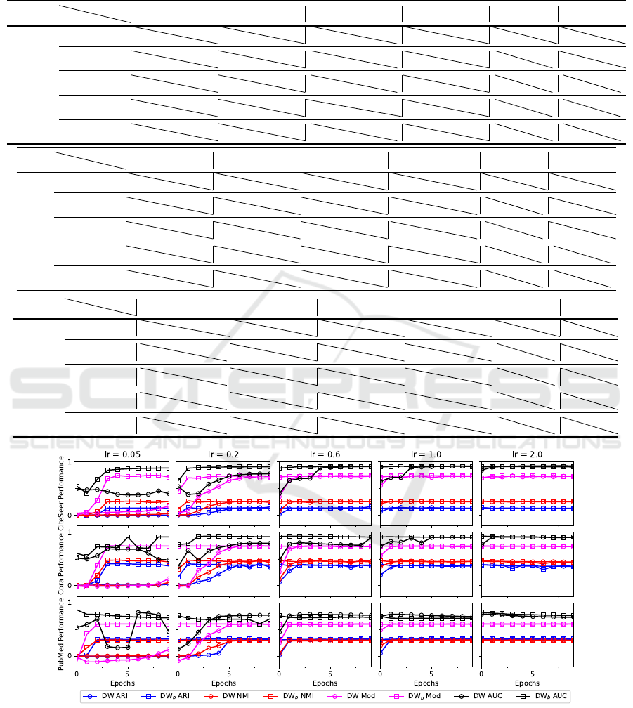
Table 2: The best performances of n2v and n2v

regarding the metrics ARI, NMI, Mod and AUC. The columns cd epochs

and lp epochs contain the required number of epochs in order for the community detection metrics (i.e. ARI, NMI, Mod) and

link prediction metric (AUC) to converge.

n2v

ARI NMI Mod AUC cd epochs lp epochs

CiteSeer

η = 0.05

0.003

0.1368

0.032

0.2634

0.1714

0.7483

0.4971

0.8861

>10

η = 0.2

0.1431

0.1567

0.2603

0.2709

0.7312

0.7334

0.7780

0.9079

>10

η = 0.6

0.1341

0.1624

0.2561

0.2617

0.7330

0.7404

0.9166

0.9129

η = 1.0

0.1471

0.1377

0.2631

0.2584

0.7376

0.74116

0.9230

0.9170

η = 2.0

0.1430

0.1411

0.2674

0.2600

0.7309

0.7354

0.9258

0.9120

n2v

ARI NMI Mod AUC cd epochs lp epochs

Cora

η = 0.05

0.0261

0.4114

0.0608

0.4789

0.1297

0.7475

0.6839

0.9147

>10

η = 0.2

0.4102

0.4085

0.4569

0.4772

0.7489

0.7446

0.7968

0.9266

>10

η = 0.6

0.4018

0.4035

0.4669

0.4710

0.7440

0.7402

0.9041

0.9281

η = 1.0

0.3838

0.4001

0.4621

0.4667

0.7448

0.7442

0.9119

0.9173

η = 2.0

0.3917

0.4085

0.4594

0.4772

0.7469

0.7446

0.9125

0.9284

n2v

ARI NMI Mod AUC cd epochs lp epochs

PubMed

η = 0.05

-0.0004

0.3185

0.0004

0.3016

0.1253

0.6014

0.8161

0.8669

>10

η = 0.2

0.3087

0.3201

0.2962

0.2996

0.6004

0.6028

0.7669

0.7535

η = 0.6

0.3139

0.3183

0.3014

0.2997

0.6013

0.5992

0.7803

0.7533

η = 1.0

0.3162

0.3200

0.3032

0.2998

0.6023

0.6016

0.7853

0.7533

η = 2.0

0.3162

0.3199

0.3034

0.2997

0.6013

0.6004

0.7856

0.8212

Figure 5: The performances of n2v and n2v

in community detection and link prediction task, considering the CiteSeer, Cora

and PubMed datasets, for different values of learning rate.

est AUC score for n2v is equal to 0.9125 (η = 2.0).

Finally, in the Pubmed graph, the highest AUC score

for n2v

is equal to 0.8669 (η = 0.05), while for n2v

is equal to 0.8161 (η = 0.05).

4 CONCLUSIONS

The aim of this paper was to improve the SkipGram

model so that it converges faster. To that end, the sig-

DeLTA 2022 - 3rd International Conference on Deep Learning Theory and Applications

moid b function with the additional trainable param-

eter b was introduced to tackle the limitations of the

standard sigmoid function used in the negative sam-

pling process. The improved update equations of the

SkipGram

model were used in the processes of DW

and n2v for generating graph embeddings, while the

k-means algorithm and the logistic regression model

were utilised to detect the communities of the graph

and to predict links between the nodes, respectively,

using the (calculated) embedded nodes. The experi-

mental results in real datasets showed that DW

and

n2v

converged faster than DW and n2v, respectively,

and attained higher ARI, Mod and AUC score in

the CiteSeer graph, as well as higher AUC score in

the Cora and PubMed graphs. Finally, the proposed

SkipGram

provided a more robust performance in

convergence speed than the standard SkipGram algo-

rithm, considering different values of learning rates.

ACKNOWLEDGEMENTS

This research is part of projects that have received

funding from the European Union’s H2020 research

and innovation programme under AIDA (GA No.

883596) and CREST (GA No. 833464).

REFERENCES

Banerjee., K., C.., V., Gupta., R., Vyas., K., H.., A., and

Mishra., B. (2021). Exploring alternatives to soft-

max function. In Proceedings of the 2nd International

Conference on Deep Learning Theory and Applica-

tions - DeLTA,, pages 81–86. INSTICC, SciTePress.

Cai, H., Zheng, V. W., and Chang, K. C.-C. (2018). A com-

prehensive survey of graph embedding: Problems,

techniques, and applications. IEEE Transactions on

Knowledge and Data Engineering, 30(9):1616–1637.

Cavallari, S., Zheng, V. W., Cai, H., Chang, K. C.-C., and

Cambria, E. (2017). Learning community embed-

ding with community detection and node embedding

on graphs. In Proceedings of the 2017 ACM on Con-

ference on Information and Knowledge Management,

pages 377–386.

Chowdhary, K. (2020). Natural language processing. In

Fundamentals of Artiﬁcial Intelligence, pages 603–

649. Springer.

Fawcett, T. (2006). An introduction to roc analysis. Pattern

recognition letters, 27(8):861–874.

Goyal, P. and Ferrara, E. (2018). Graph embedding tech-

niques, applications, and performance: A survey.

Knowledge-Based Systems, 151:78–94.

Grover, A. and Leskovec, J. (2016). node2vec: Scal-

able feature learning for networks. In Proceedings

of the 22nd ACM SIGKDD international conference

on Knowledge discovery and data mining, pages 855–

864.

Hartigan, J. A. and Wong, M. A. (1979). Algorithm as

136: A k-means clustering algorithm. Journal of the

royal statistical society. series c (applied statistics),

28(1):100–108.

He, T., Zhang, Z., Zhang, H., Zhang, Z., Xie, J., and Li,

M. (2019). Bag of tricks for image classiﬁcation

with convolutional neural networks. In Proceedings

of the IEEE Conference on Computer Vision and Pat-

tern Recognition, pages 558–567.

Hochreiter, S. (1998). The vanishing gradient problem dur-

ing learning recurrent neural nets and problem solu-

tions. International Journal of Uncertainty, Fuzziness

and Knowledge-Based Systems, 6(02):107–116.

Hosmer Jr, D. W., Lemeshow, S., and Sturdivant, R. X.

(2013). Applied logistic regression, volume 398. John

Wiley & Sons.

Luo, X., Chang, X., and Ban, X. (2016). Regression and

classiﬁcation using extreme learning machine based

on l1-norm and l2-norm. Neurocomputing, 174:179–

186.

Mikolov, T., Chen, K., Corrado, G., and Dean, J. (2013a).

Efﬁcient estimation of word representations in vector

space. arXiv preprint arXiv:1301.3781.

Mikolov, T., Sutskever, I., Chen, K., Corrado, G. S., and

Dean, J. (2013b). Distributed representations of words

and phrases and their compositionality. Advances

in neural information processing systems, 26:3111–

3119.

Nguyen, G. H., Lee, J. B., Rossi, R. A., Ahmed, N. K., Koh,

E., and Kim, S. (2018). Continuous-time dynamic net-

work embeddings. In Companion Proceedings of the

The Web Conference 2018, pages 969–976.

Perozzi, B., Al-Rfou, R., and Skiena, S. (2014). Deepwalk:

Online learning of social representations. In Proceed-

ings of the 20th ACM SIGKDD international confer-

ence on Knowledge discovery and data mining, pages

701–710.

Rozemberczki, B., Davies, R., Sarkar, R., and Sutton, C.

(2019). Gemsec: Graph embedding with self clus-

tering. In Proceedings of the 2019 IEEE/ACM inter-

national conference on advances in social networks

analysis and mining, pages 65–72.

Sen, P., Namata, G., Bilgic, M., Getoor, L., Galligher, B.,

and Eliassi-Rad, T. (2008). Collective classiﬁcation in

network data. AI magazine, 29(3):93–106.

Vinh, N. X., Epps, J., and Bailey, J. (2010). Information the-

oretic measures for clusterings comparison: Variants,

properties, normalization and correction for chance.

The Journal of Machine Learning Research, 11:2837–

2854.

Zhang, D., Yin, J., Zhu, X., and Zhang, C. (2018). Network

representation learning: A survey. IEEE transactions

on Big Data.

A Faster Converging Negative Sampling for the Graph Embedding Process in Community Detection and Link Prediction Tasks