Calibration of a 2D Scanning Radar and a 3D Lidar

Jan M. Rotter and Bernardo Wagner

Real Time Systems Group, Leibniz University of Hanover, Appelstraße 9a, 30167 Hanover, Germany

Keywords:

Mobile Robotics, 2D Scanning Radar, 3D Lidar, Target-less Calibration, Search and Rescue Robotics.

Abstract:

In search and rescue applications, mobile robots have to be equipped with robust sensors that provide data

under rough environmental conditions. One such sensor technology is radar which is robust against low-

visibility conditions. As a single sensor modality, radar data is hard to interpret which is why other modalities

such as lidar or cameras are used to get a more detailed representation of the environment. A key to successful

sensor fusion is an extrinsically and intrinsically calibrated sensor setup. In this paper, a target-less calibration

method for scanning radar and lidar using geometric features in the environment is presented. It is shown

that this method is well-suited for in-ﬁeld use in a search and rescue application. The method is evaluated

in a variety of use-case relevant test scenarios and it is demonstrated that the calibration results are accurate

enough for the target application. To validate the results, the proposed method is compared to a target-based

state-of-the-art calibration method showing equivalent performance without the need for specially designed

targets.

1 INTRODUCTION

A civil use-case of autonomous robots is search and

rescue (SAR) (Kim et al., 2015) (Fritsche et al., 2017)

(Fan et al., 2019). In disaster situations, ﬁrst respon-

ders need to act as quickly as possible while protect-

ing their own life. SAR robots provide a means to get

an overview of a situation or to search for survivors

in places that are not reachable by human helpers.

Usually, disaster sites are considered harsh and chal-

lenging environments. They can be covered in dust

or smoke with objects lying or hanging around and

blocking the path of an autonomous robot. Therefore,

SAR robots are equipped with robust sensor modali-

ties. To recognize smaller objects, a high-resolution

lidar or camera could be used. But these modali-

ties lose precision in smoke or dust since a visual

line of sight to the target is needed. To ensure ba-

sic operation, radar can be used as an additional sen-

sor that is robust against these disturbances but is not

as precise as visual sensor modalities (Fritsche et al.,

2017). To maximize information value, sensor read-

ings from multiple modalities can be fused (Fritsche

et al., 2016). Essential for sensor fusion is an ex-

trinsic and intrinsic calibration providing translation

and rotation between the sensors as well as any scal-

ing or offset parameters inherent to a speciﬁc sen-

https://orcid.org/0000-0001-5900-0935

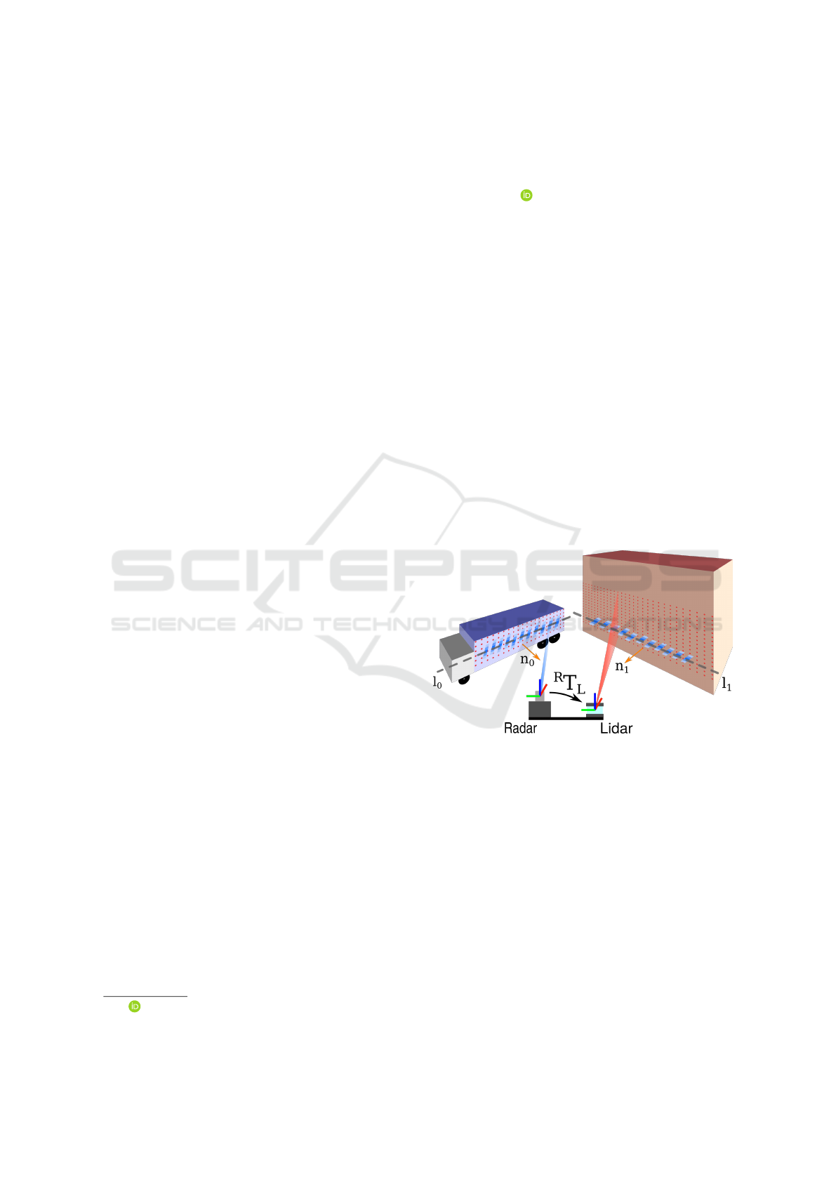
Figure 1: Schematic of the proposed in-ﬁeld calibration

method for search and rescue robots.

sor. There exist multiple methods to calibrate a sensor

setup. Manual measurement can only provide an ap-

proximation since in most cases the sensor’s origin is

unknown. Also, intrinsic parameters can be hard or

even impossible to measure. External measurement

tools like laser trackers or optical tracking systems

provide higher precision in determining the extrinsic

parameters while the direct extraction of intrinsic pa-

rameters remains problematic. To ﬁnd an extrinsic

and also intrinsic set of calibration parameters, cor-

responding sensor readings between two sensors can

be used. These methods can be divided into target-

based and target-less methods. The target-based cal-

ibration uses carefully designed targets that are easy

Rotter, J. and Wagner, B.

Calibration of a 2D Scanning Radar and a 3D Lidar.

DOI: 10.5220/0011140900003271

In Proceedings of the 19th International Conference on Informatics in Control, Automation and Robotics (ICINCO 2022), pages 377-384

ISBN: 978-989-758-585-2; ISSN: 2184-2809

377

to detect in all sensor modalities. Time-synchronized

detections are used as correspondences and the dis-

tances between detections are minimized over all cor-

respondences. In contrast, target-less methods only

use corresponding features detected in the environ-

ment. In SAR applications only manual or target-less

calibration can be used. Although target-based meth-

ods could be used in the ﬁeld, they are impractical due

to the calibration targets that require additional pack-

aging space. Moreover, target-based methods usually

take a longer time when the calibration target has to

be moved to several different positions. External cal-

ibration tools can only be used when the sensor setup

is never changed. This cannot be ensured since equip-

ment may be disassembled for minimized packaging

space. In this paper, an efﬁcient target-less calibra-

tion method for 2D scanning radar and 3D lidar is

presented. In contrast to the few other target-less ap-

proaches to this problem, calibrating the intrinsic off-

set parameter that exists in most scanning radar sen-

sors is additionally considered. As calibration fea-

tures, geometric primitives like planes and lines that

can be found in a structured or semi-structured envi-

ronment are used.

2 RELATED WORKS

Radar as a sensor modality in mobile robotics has re-

cently become more popular. Over time various cali-

bration methods for different sensor setups have been

developed. The applied techniques mainly use target-

based methods although a few target-less approaches

exist.

2.1 Target-based Methods

Sugimoto et al. determine the extrinsic parameters

between a monocular camera and a static 2D radar.

A single corner reﬂector is used as a calibration tar-

get which is moved perpendicular to the radar plane.

Local maxima in the radar measurements are consid-

ered to be crossing points of the reﬂector and radar

plane where a corresponding camera measurement is

recorded. All corresponding measurements are used

in a least-squares estimation to calculate the extrinsic

calibration (Sugimoto et al., 2004). Wang et al. use a

similar approach but with a sheet of metal as a calibra-

tion target which is detected in both camera and radar.

To ﬁlter the measurements a clustering algorithm is

applied to the target detections (Wang et al., 2011).

El Natour et al. are the ﬁrst to relax the zero-elevation

assumption of radar measurements. They take into ac-

count that not every radar measurement is located in

the center of the measurement cone. Therefore, a 3D

point detected in both camera and radar is modeled as

the intersection of the light ray passing through this

point and the camera center with a sphere centered

at the radar center. The sensor setup is moved around

multiple corner targets and the trajectory of the move-

ment is used in the optimization process (El Natour

et al., 2015). Per

c et al. present a calibration target

that can be used for camera, lidar, and radar calibra-

tion simultaneously based on a corner reﬂector behind

a triangular-shaped styrofoam plane with a checker-

board pattern. For the extrinsic calibration between li-

dar and radar, the radar cross-section (RCS) is used to

estimate the elevation angle of the reﬂected radar sig-

nals and to reﬁne the Z-axis parameter (Per

c et al.,

2017) (Per

c et al., 2019). Domhof et al. use a tar-

get design consisting of a styrofoam plane with four

circular holes and a corner reﬂector in the center for

camera, lidar, and radar calibration. In contrast to El

Natour et al., radar detections are considered to lie on

a 2D plane. In their experiments, it is shown that the

Root Mean Square Error (RMSE) is approximately

2 cm for the lidar-to-radar calibration and 2.5 cm for

the camera-to-radar calibration (Domhof et al., 2019).

In a follow-up work, experiments to evaluate different

calibration constraints, as well as relative and absolute

calibration results are added (Domhof et al., 2021).

2.2 Target-less Methods

Sch

oller et al. introduce a data-driven method to cal-

ibrate a camera-radar-system without calibration tar-

gets. They train two neural networks in a boosting-

inspired algorithm to estimate the rotational calibra-

tion parameters. The euclidean distance between the

estimated and true quaternion is used as loss function

(Scholler et al., 2019). To calibrate a system of multi-

ple laser scanners and automotive radar sensors, Heng

uses a previously built map to ﬁrst calibrate the laser

scanners to each other. In a second step, the point-

to-plane distance of the radar target detections to the

mapped points is minimized (Heng, 2020). A differ-

ent approach is used by Wise et al. In their work,

velocity vectors from a camera-radar setup are ex-

tracted from the sensor data for each sensor individ-

ually which are used to estimate the extrinsic param-

eters (Wise et al., 2021). Per

c et al. also present a

target-less calibration method that can be used as a de-

calibration detection as well. In every sensor modal-

ity, features are detected and tracked individually to

obtain the sensor’s trajectory. An association algo-

rithm is used to ﬁnd differences between the differ-

ent sensor paths. If deviations are detected, a graph-

based calibration towards one anchoring sensor is per-

ICINCO 2022 - 19th International Conference on Informatics in Control, Automation and Robotics

378

formed. The authors state that the method is limited to

rotational calibration and decalibration detection only

(Per

c et al., 2021).

2.3 Contribution

In this paper, a target-less calibration method based

on geometric primitives is presented. It is specially

designed for in-ﬁeld use in the SAR domain. Unlike

all previously mentioned works, a scanning radar is

employed instead of ﬁxed n-channel sensor modules.

Additionally, the internal offset parameter which is

introduced by the rotating mirror as well as electri-

cal signal delays is optimized. Raw range proﬁles

are used instead of previously extracted target detec-

tions common to commercial automotive radar mod-

ules. Feature detection is applied to both radar and

lidar to extract geometric primitives in both modali-

ties. The calibration is modeled as a graph optimiza-

tion problem. To ensure a good calibration quality,

ﬁltering methods to collect features with a greater va-

riety via azimuth and elevation binning are applied.

Evaluation is provided to analyze the absolute cali-

bration error which is compared to the results of the

target-based method by Per

c et al.

3 METHODOLOGY

The calibration method consists of a three-step pre-

processing, matching, and optimization pipeline.

First, raw sensor data is ﬁltered to extract the relevant

points from the radar and lidar respectively. Second,

features from different sensor modalities are assigned

to each other to build the constraints used in the op-

timization. Last, the set of constraints is ﬁltered to

keep informative matches and graph optimization is

used to estimate the parameters.

3.1 Assumptions

Both sensors have to be synchronized in time. This

is necessary to assign a corresponding lidar scan to

each radar scan. Also, velocities of sensor movements

are assumed to be slow enough that motion correction

can be omitted. Finally, a set of initial calibration pa-

rameters is needed to transform the points into one

common coordinate frame. The method mainly ap-

plies to FMCW radar sensors with a rotating mirror,

although it may be used with other radar sensors as

well for example by constraining the distance offset

parameter to zero. For the proposed method the radar

data consists of uncalibrated range proﬁles of which

the range resolution has to be known in advance. The

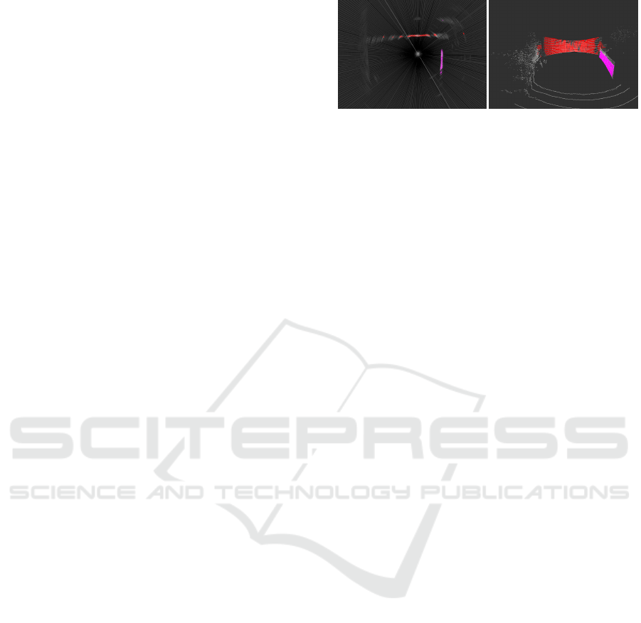
(a) Radar scan.

(b) Lidar scan.

Figure 2: Visualization of processed sensor data from an

outdoor data set. (a): Raw radar data (black/white) and de-

tected lines (colored). (b): Raw lidar data (white) and de-

tected planes (colored). A photo of the scene can be seen in

Figure 6f.

resolution can be calculated from the bandwidth and

the analog-digital-converter parameters of the sensor.

3.2 Preprocessing

The ﬁrst step is to process the data of each sensor in-

dividually to extract the features used in the matching

and optimization step. Starting with the radar sen-

sor, each scan is ﬁltered by a standard CA-CFAR ﬁlter

(Keel, 2010) that has to be tuned manually to the sen-

sor’s dynamic range. This removes noise and most of

the clutter from the radar signal so that only potential

target points including multi-path reﬂections remain.

Since valid target points behind walls or other obsta-

cles would not be seen by the lidar, all radar target

detections behind the ﬁrst one are removed. This also

reduces multi-path reﬂections to a minimum. Then a

RANSAC model (Fischler and Bolles, 1981) is used

to search for lines in the radar target points which

are highly likely to be found in structured and semi-

structured environments. The distance for a point to

be considered an inlier to a line is set to a more tol-

erant value compared to what would be necessary for

lidar points since the results of the CFAR ﬁlter are

not as accurate as lidar data. This results in a set of

line parameters and their corresponding inlier points.

Figure 2a shows the raw radar sensor data (black &

white) as well as the extracted line points (colored).

The lidar data is ﬁrst processed by a statistical out-

lier ﬁlter to remove very small objects or erroneous

measurements. After using a voxel grid ﬁlter, a range

image of the point cloud is created. To ﬁnd large

homogeneous regions which are typical for planes in

structured environments, the magnitude of the gradi-

ents in the range image is calculated and ﬁltered by

a threshold. The remaining point locations involve

only limited changes in the range between neighbor-

ing points. To reﬁne the regions, a distance transform

is applied and all points in the border areas of the ho-

mogeneous regions are removed. The range image is

Calibration of a 2D Scanning Radar and a 3D Lidar

379

Figure 3: Matching of detected lidar planes P

to a radar

line represented by a helper plane P

then transformed back into a point cloud. To achieve

a more robust plane ﬁtting, ground segmentation is

performed and the potential ground plane is removed.

In this reduced lidar cloud, planes that are perpendic-

ular to the radar plane up to an angle ε are extracted.

This angle should be chosen big enough, for example,

ε = 45

◦

, so that also tilted planes from the environ-

ment intersecting with the radar plane are recognized.

A RANSAC model is used for the plane extraction,

too. The result of the plane search can be seen in

Figure 2b where raw lidar points are white and the

identiﬁed planes are indicated by different colors.

3.3 Matching

Processing both sensor modalities results in a set of

line parameters and corresponding radar target points

as well as a set of plane parameters with their corre-

sponding lidar points. To ﬁnd matches between these

two sets, ﬁrst, the parameters of a helper plane P

per-

pendicular to the radar measurement plane are cal-

culated for each detected radar line. For each lidar

plane P

, the normal vector is projected onto the radar

measurement plane. Then the intersection point be-

tween the projected normal vector and the detected li-

dar plane is determined. A correspondence is formed

by a plane-line pair where the distance d

between the

normal intersection point of the radar helper plane and

the intersection point calculated for the lidar plane is

minimal. A visualization of the matching step is given

in ﬁgure 3. This ensures that direction, as well as

distance, are taken into account and also that heav-

ily tilted lidar planes can be matched to a radar line

detection. To ensure proper distribution of correspon-

dences over the whole sensing area, all correspon-

dences are assigned to an azimuth and elevation bin

based on the respective angles of the lidar plane’s nor-

mal vector. Correspondence samples are collected un-

til at least N samples are recorded for every bin com-

bination.

Figure 4: System overview.

3.4 Optimization

Scanning radars use a spinning mirror above the trans-

mitter/receiver antenna. This leads to a distance off-

set in the raw sensor data o

as depicted in Fig-

ure 4. The internal signal paths between the sig-

nal generator, antenna, and the A/D-converter in-

crease this distance offset. Therefore, additionally to

the extrinsic calibration parameters, the distance off-

set is optimized. The optimization problem is mod-

eled as a graph with only one optimizable vertex v

which holds the calibration parameters using the g2o-

framework (Kummerle et al., 2011). For every line-

to-plane-correspondence, the lidar plane parameters

are inserted as non-optimizable vertices v

. For every

radar line point, an edge deﬁning the measurement of

the radar error as

e(n

, p

, o

) = n

∗

−1

∗



+ o

∗



(1)

is inserted between the parameter vertex v

and the

correspondence vertex v

effectively minimizing the

point-to-plane distance. Here n

is the plane normal of

the laser plane, p

is the point from the corresponding

radar line,

is the 3D transformation matrix from

the radar to the lidar coordinate frame and o

is the

intrinsic radar offset parameter.

The uncertainty of the radar measurements which

originates from two sources is also modeled. First,

in FMCW radar the continuous signals are sampled

and discretized by the A/D converter. This discretiza-

tion through the sampling rate into ﬁxed-sized bins

deﬁnes the range resolution and is used as the range

uncertainty. Second, the expansion of the transmitted

radar signal depends highly on the antenna used in the

sensor module. Antennas form the shape of the main

and side lobes of the radar beam. The ﬁeld of view of

the radar beam is deﬁned as the −3 dB range of the

main lobe and can be modeled as a cone. The uncer-

tainty of the azimuth and elevation angle is therefore

ICINCO 2022 - 19th International Conference on Informatics in Control, Automation and Robotics

380

set to the size of the ﬁeld of view. At 0°azimuth, this

results in a covariance matrix of

(d) =





bin

0 0

0 (d tanα

f ov

)

0 0 (d tanα

f ov

)





(2)

with range bin size s

bin

, range measurement d =

and ﬁeld of view angle α

f ov

. For other azimuth or in

the general case elevation angles the respective rota-

tion has to be applied.

4 EXPERIMENTS

To validate the method and to compare it to meth-

ods from the state-of-the-art, multiple experiments are

conducted using a Velodyne VLP-16 Puck as a laser

scanner and two different scanning radars (Navtech

CIR204, Indurad iSDR-C). The laser scanner uses 16

rays in its vertical ﬁeld of view of 30°at a horizon-

tal resolution of 0.3°. The Navtech radar has a beam

opening angle of 1.8°, a horizontal resolution of 0.9°,

and a range resolution of 0.06 m, whereas the Indurad

radar has a beam opening angle of about 3°at a similar

horizontal resolution and a range resolution of 0.04 m.

All sensors have a horizontal ﬁeld of view of 360°.

Three different sensor setups which are shown in Fig-

ure 5 are used. In the ﬁrst setup (a) the Indurad radar

and the Velodyne lidar are mounted on top of each

other on a handheld sensor frame to provide a better

motion radius and to verify that the method can pro-

vide a reasonably good lidar-to-radar calibration. For

a second experiment, the same sensor setup is placed

underneath a UAV platform (b) that could be used

in a search and rescue scenario. The UAV is moved

and tilted manually with two persons to show that the

method works in a real-world scenario and can speed

up the calibration process in an emergency situation.

The last setup (c) is built onto an UGV platform us-

ing the Navtech radar along with the Velodyne lidar.

In this setup, a greater distance between the sensors is

chosen to ﬁnd out how the method deals with fewer

constraints through movement and rotation. For all

setups, ground truth for the extrinsic 6-DOF parame-

ter set is measured. The ground truth information for

the ﬁrst two setups is extracted from CAD models.

To obtain ground truth parameters for the third setup,

an optical tracking system is used to measure trans-

lation and rotation between the sensors on the mobile

platform. To determine the internal offset parameter,

the distance between the center of the radome and a

single corner reﬂector is ﬁrst measured by using the

tracking system and then by detecting the reﬂector in

the radar scan. The difference between both measure-

ments is used as ground truth offset. All ground truth

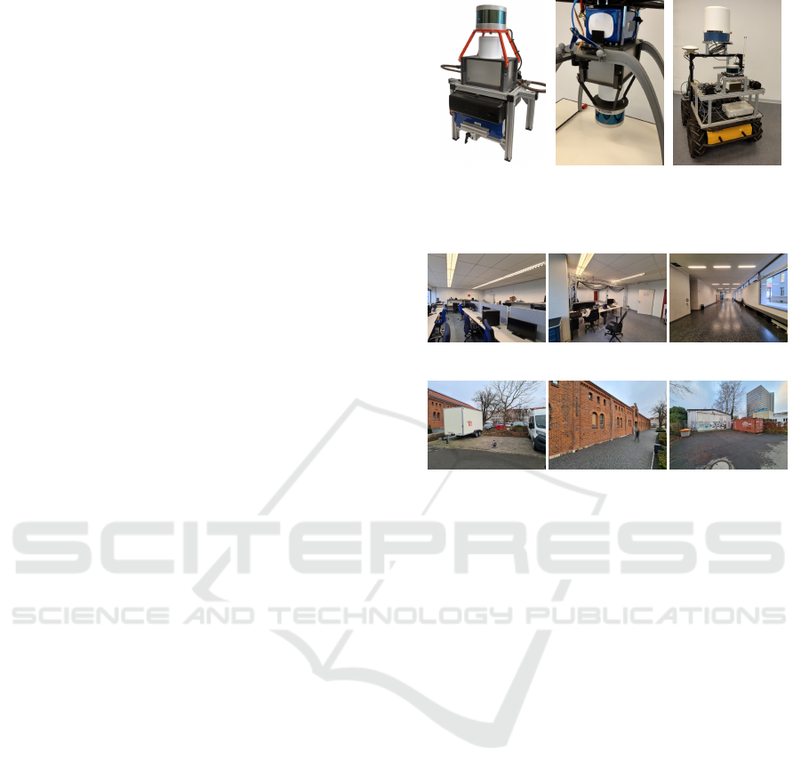
(a) (b) (c)

Figure 5: Sensor setups used in the experiments. Handheld

sensor box (a), UAV (b) and (c) UGV mounted setups.

(a) (b) (c)

(d) (e) (f)

Figure 6: Indoor sites (a - c) and outdoor scenarios (d - f).

‘

calibration parameters are provided in Table 1. The

handheld setup (a) is used in different environments to

gather test data. The ﬁrst testing sites are lab environ-

ments as they provide at least two clean and perpen-

dicular walls which are expected to be easy to extract

as planes. Since the labs are only normal-sized rooms

a wider lobby-like location is added to the dataset.

Furthermore, outdoor data is collected between two

vans on a parking lot, in front of a building, and in a

corner between a building and an overseas container.

These sites were chosen because of their use-case-

related nature. The different indoor testing sites can

be seen in Figures 6a-6c and the outdoor sites are de-

picted in Figures 6d-6f. The data for setups (b) and

compare the ﬁndings to the state-of-the-art a calibra-

tion using a target similar to (Domhof et al., 2019)

and the optimization method of (Per

c et al., 2019)

is implemented and extended by an internal offset pa-

rameter optimization.

5 RESULTS

For each of the experimental setups, the calibration is

estimated 50 times on a recorded data set to test accu-

racy and reliability. In each setup, the same set of pa-

Calibration of a 2D Scanning Radar and a 3D Lidar

381

Table 1: Ground truth and initial calibration parameters for all setups.

[m] t

[m] o[m] r

[

◦

] r

[

◦

] r

[

◦

]

Ground Truth

Handheld (a) 0.0 0.0 0.095 0.175 0.0 0.0 -145.6

UAV (b) 0.0 0.0 0.095 0.175 0.0 0.0 0.0

UGV (c) 0.371 -0.006 -0.402 0.409 0.00 0.01 0.01

Initial

Handheld (a) 0.0 0.0 0.0 0.0 0.0 0.0 -132.0

UAV (b) 0.0 0.0 0.0 0.0 0.0 0.0 0.0

UGV (c) 0.3 0.0 -0.5 0.0 0.0 0.0 0.0

Table 2: Mean and standard deviation of estimated parameters (n = 50) in all calibration scenarios.

[m] t

[m] o[m] R

yaw

[

◦

] R

pitch

[

◦

] R

roll

[

◦

]

Lab 1

µ -0.005 -0.005 0.074 -0.19 -143.275 -0.741 0.927

σ 0.03 0.034 0.045 0.018 0.942 2.134 1.794

Lab 2

µ 0.014 -0.018 0.089 -0.246 -142.508 0.109 1.357

σ 0.046 0.038 0.05 0.032 1.449 1.871 1.445

Lobby

µ 0.017 -0.002 0.075 -0.215 -143.707 -6.294 5.518

σ 0.035 0.037 0.09 0.016 0.713 3.424 2.924

Parked Cars

µ -0.01 -0.067 0.072 -0.124 -146.099 -2.833 3.752

σ 0.056 0.066 0.203 0.032 2.055 9.618 8.593

1 Wall

µ 0.003 -0.009 0.032 -0.181 -143.104 1.837 0.677

σ 0.035 0.041 0.127 0.019 0.702 4.237 3.965

2 Walls

µ -0.005 -0.002 0.05 -0.168 -146.177 -0.042 -0.056

σ 0.021 0.022 0.061 0.013 0.427 1.253 1.389

UAV

µ 0.008 0.0 0.142 -0.27 -3.568 -1.274 -0.259

σ 0.014 0.019 0.052 0.015 0.536 1.79 1.5

UGV

µ 0.325 0.033 -0.148 -0.569 0.888 2.998 -1.836

σ 0.032 0.064 0.32 0.025 0.519 3.503 7.239

Table 3: Mean estimated parameter uncertainty (n = 50) of all calibration scenarios.

[m] t

[m] o[m] R

yaw

[

◦

] R

pitch

[

◦

] R

roll

[

◦

]

Lab 1 0.127 0.116 0.192 0.105 0.983 2.607 2.323

Lab 2 0.124 0.113 0.172 0.094 1.377 1.972 2.174

Lobby 0.073 0.068 0.128 0.06 0.232 0.597 0.563

Parked Cars 0.121 0.105 0.258 0.098 0.586 1.337 2.617

1 Wall 0.072 0.064 0.187 0.064 0.13 0.702 0.659

2 Walls 0.08 0.091 0.181 0.07 0.56 1.87 1.913

UAV 0.117 0.136 0.209 0.095 1.721 3.242 3.071

UGV 0.089 0.091 0.506 0.081 0.549 3.429 3.757

Table 4: Absolute calibration errors for state-of-the-art and our method (means).

Method e

[m] e

[

◦

] e

[

◦

] e

[

◦

] e

[m]

Per

c et al. 0.031 0.009 0.078 0.005 0.012 0.004 0.11

Ours (Handheld, best) 0.003 0.002 0.005 0.056 0.042 0.577 0.006

Ours (Handheld, worst) 0.017 0.067 0.063 5.518 6.294 3.092 0.071

Ours (UAV) 0.008 0.0 0.047 0.259 1.274 3.568 0.1

Ours (UGV) 0.046 0.039 0.254 1.836 2.988 0.007 0.16

rameters for the input ﬁltering as well as for matching

and binning consisting of three azimuth times three

elevation bins (< −6

◦

, [−6

◦

, 6

◦

), ≥ 6

◦

) is used. Per

bin, N = 15 plane-to-line matches are extracted for

optimization. The only difference between the exper-

iments is the initial calibration which has to match

the individual sensor setup and is determined by man-

ual measurement. Table 1 provides the initial pa-

rameters. For each optimization, the estimated per-

parameter uncertainty is extracted by calculating the

ICINCO 2022 - 19th International Conference on Informatics in Control, Automation and Robotics

382

standard deviation from the information matrix used

in the graph optimization.

Table 2 shows the mean and the measured stan-

dard deviation of the estimated calibration parame-

ters. Independent of the scenario rotational param-

eters are estimated within a narrow region around

ground truth with the only exception being the lobby

data set. The same applies to XY-translation and

the internal offset parameter. The measured per-

parameter standard deviation over all calibration runs

shows that most results lie in a region around the

mean value of 3 cm to 5 cm or 2°to 4°respectively.

Only Z-translation shows a wide range of optimiza-

tion results. This is expectable for the chosen sen-

sor setups: Z-estimation improves only with high an-

gles of the extracted planes in the lidar data. Using

only 16 vertical scans, a heavily tilted plane produces

a sparser point cloud which makes plane estimation

less reliable compared to a perpendicular plane. This

can easily lead to a sparse set of constraints or erro-

neous plane extractions and could be the reason for

the slightly worse calibration results of XY-rotation

parameters in the lobby data set. The outdoor data

suggests that using two parked cars as calibration tar-

gets is a more difﬁcult scenario. Despite good de-

tectability of the metal surfaces in radar data, the

plane detection in lidar data gets distorted through

the non-optimal shape of the vehicle which leads to

a higher deviation in almost all parameters. How-

ever, using one or two walls as calibration features

produces accurate results, except for the problematic

Z-translation, which suggests applicability in the tar-

get scenario.

Applicability is also the motivation for the exper-

iments with the UAV and UGV platforms. Using the

UAV platform, two operators are able to perform cal-

ibration by carrying the robot while rotating and dis-

placing it in front of the calibration features. Gather-

ing all the necessary samples takes less than ﬁve min-

utes additional to the three minutes of optimization

runtime on a current laptop CPU.

Since free movement in 6-DOF space is not possi-

ble for every sensor setup or robotic application (e.g.

think about autonomous driving), an additional exper-

iment is conducted with a UGV platform. By using

ramps to ensure at least a limited rotation around the

X- and Y-axis, the binning parameters from before

can not be used. Instead, ﬁve azimuth bins and no

elevation binning are conﬁgured. The results show

that the accuracy in most parameters suffers without

the necessary constraints in elevation. Especially ro-

tation estimation around the X- and Y-axis gets more

inaccurate with a standard deviation of up to 7°. The

greatest discrepancies can be seen in Z-translation

with a standard deviation around 0.3 m. Partly these

discrepancies can be explained by the lower range res-

olution of the Navtech radar sensor of 0.06 m but this

experiment shows the necessity of the 6-DOF move-

ment for this calibration method.

Another important measure is the uncertainty esti-

mation of the optimization process. Table 3 shows the

estimated per-parameter uncertainty for all calibration

scenarios. For all translational parameters, this esti-

mation exceeds the actual standard deviations while

this is not the case for all the rotation uncertainties.

This shows that the assumed error model is not accu-

rate enough to estimate the uncertainty precisely. For

example, the error stemming from plane estimation is

not modeled in the uncertainty estimation.

To compare the proposed method with the current

state-of-the-art target-based method of (Per

c et al.,

2017) the UGV sensor setup is used for data acquisi-

tion. It is not necessary to move the sensor setup since

the calibration target is moved instead. Therefore, the

aforementioned problems are not relevant to this ex-

periment. Table 4 lists the absolute calibration error

for all experiments. For the comparison, the mean

parameter values of the proposed method are used to

determine the error. Data shows that the target-less

method can compete with the state-of-the-art target-

based method or in the best case even outperform it.

All the more, when looking at the worst-case abso-

lute errors similar accuracy in translation and intrinsic

offset is achieved. Only rotation around the X- and Y-

axis are less accurate, although both worst-case esti-

mations stem from the indoor lobby data set. Overall,

using the target-less method results in more accurate

translation parameters whereas rotation is better esti-

mated by the target-based method.

6 CONCLUSION AND FUTURE

WORK

Search and rescue robotics demands techniques that

are easily applicable in the ﬁeld without the need

for additional hardware or high-precision equipment.

This work shows that it is possible to successfully cal-

ibrate a 3D lidar to a 2D scanning radar by only using

geometrical features from the environment. An ac-

ceptable accuracy regarding absolute calibration error

which mostly lies within the discretization accuracy

of the radar sensors can be achieved. Only transla-

tion along the Z-axis is not estimated well enough.

Besides the Z-axis-aligned sensor setup, plane extrac-

tion accuracy has a major impact on the optimization

of that parameter. In such a setup, only heavily tilted

planes introduce the necessary constraints to better es-

Calibration of a 2D Scanning Radar and a 3D Lidar

383

timate the Z-translation. In comparison to the state-

of-the-art, the proposed method achieves comparable

results while not using any artiﬁcial calibration tar-

gets. This makes the method versatile and applicable

in search and rescue scenarios.

In the future, one goal will be the reduction of

erroneous plane extractions which add inconclusive

constraints to the optimization process. Reducing

such mismatches directly improves the parameter es-

timation and also has a positive effect on the repeat-

able accuracy. Additional error modeling of the plane

extraction process will also improve uncertainty esti-

mation. Furthermore, using bins not only for azimuth

and elevation but also for the distance of the plane-

line-matches could be beneﬁcial for the optimization

result.

ACKNOWLEDGEMENTS

This work has partly been funded by the German Fed-

eral Ministry of Education and Research (BMBF) un-

der the project number 13N15550 (UAV-Rescue).

REFERENCES

Domhof, J., Kooij, J. F., and Gavrila, D. M. (2021). A

Joint Extrinsic Calibration Tool for Radar, Camera

and Lidar. IEEE Transactions on Intelligent Vehicles,

6(3):571–582.

Domhof, J., Kooij, J. F. P., and Gavrila, D. M. (2019). A

multi-sensor extrinsic calibration tool for lidar , cam-

era and radar. IEEE International Conference on

Robotics and Automation (ICRA), pages 1–7.

El Natour, G., Ait-Aider, O., Rouveure, R., Berry, F., and

Faure, P. (2015). Toward 3D reconstruction of outdoor

scenes using an MMW radar and a monocular vision

sensor. Sensors (Switzerland), 15(10):25937–25967.

Fan, H., Bennetts, V. H., Schaffernicht, E., and Lilienthal,

A. J. (2019). Towards gas discrimination and mapping

in emergency response scenarios using a mobile robot

with an electronic nose. Sensors (Switzerland), 19(3).

Fischler, M. a. and Bolles, R. C. (1981). Random Sample

Consensus: A Paradigm for Model Fitting with Ap-

plications to Image Analysis and Automated Cartog-

raphy. Communications of the ACM, 24(6):381–395.

Fritsche, P., Kueppers, S., Briese, G., and Wagner, B.

(2016). Radar and LiDAR Sensorfusion in Low Vis-

ibility Environments. In Proceedings of the 13th In-

ternational Conference on Informatics in Control, Au-

tomation and Robotics (ICINCO), volume 2, pages

30–36. SciTePress.

Fritsche, P., Zeise, B., Hemme, P., and Wagner, B. (2017).

Fusion of radar, LiDAR and thermal information for

hazard detection in low visibility environments. SSRR

2017 - 15th IEEE International Symposium on Safety,

Security and Rescue Robotics, Conference, pages 96–

101.

Heng, L. (2020). Automatic targetless extrinsic calibration

of multiple 3D LiDARs and radars. In IEEE Interna-

tional Conference on Intelligent Robots and Systems.

Keel, B. M. (2010). Constant False Alarm Rate Detectors.

In Richards, M. A., Scheer, J. A., and Holm, W. A.,

editors, Principles of Modern Radar: Basic princi-

ples, chapter 16, pages 589–621. Institution of Engi-

neering and Technology, Edison, NJ.

Kim, J. H., Starr, J. W., and Lattimer, B. Y. (2015). Fire-

ﬁghting Robot Stereo Infrared Vision and Radar Sen-

sor Fusion for Imaging through Smoke. Fire Technol-

ogy, 51(4):823–845.

Kummerle, R., Grisetti, G., Strasdat, H., Konolige, K.,

and Burgard, W. (2011). G2o: A general framework

for graph optimization. In 2011 IEEE International

Conference on Robotics and Automation, pages 3607–

3613. IEEE.

Per

c, J., Markovi

c, I., and Petrovi

c, I. (2017). Extrinsic

6DoF calibration of 3D LiDAR and radar. 2017 Euro-

pean Conference on Mobile Robots, ECMR 2017.

Per

c, J., Markovi

c, I., and Petrovi

c, I. (2019). Extrinsic

6DoF calibration of a radar–LiDAR–camera system

enhanced by radar cross section estimates evaluation.

Robotics and Autonomous Systems, 114:217–230.

Per

c, J., Petrovi

c, L., Markovi

c, I., and Petrovi

c, I. (2021).

Online multi-sensor calibration based on moving ob-

ject tracking. Advanced Robotics, 35(3-4):130–140.

Scholler, C., Schnettler, M., Krammer, A., Hinz, G.,

Bakovic, M., Guzet, M., and Knoll, A. (2019). Target-

less Rotational Auto-Calibration of Radar and Cam-

era for Intelligent Transportation Systems. In 2019

IEEE Intelligent Transportation Systems Conference

(ITSC), pages 3934–3941. IEEE.

Sugimoto, S., Tateda, H., Takahashi, H., and Okutomi,

M. (2004). Obstacle detection using millimeter-

wave radar and its visualization on image sequence.

Proceedings - International Conference on Pattern

Recognition, 3(May):342–345.

Wang, T., Zheng, N., Xin, J., and Ma, Z. (2011). Integrating

millimeter wave radar with a monocular vision sensor

for on-road obstacle detection applications. Sensors,

11(9):8992–9008.

Wise, E., Persic, J., Grebe, C., Petrovic, I., and Kelly, J.

(2021). A Continuous-Time Approach for 3D Radar-

to-Camera Extrinsic Calibration. In 2021 IEEE In-

ternational Conference on Robotics and Automation

(ICRA), pages 13164–13170. IEEE.

ICINCO 2022 - 19th International Conference on Informatics in Control, Automation and Robotics

384