User Proﬁling: On the Road from URLs to Semantic Features

Claudio Barros and Perrine Moreau

Data Science Direction, M

ediam

etrie, 70 rue Rivay, Levallois-Perret, France

Keywords:

Text Mining, URLs, User Proﬁling, Feature Engineering, Topic Extraction, Semantics.

Abstract:

Text data is undoubtedly one of the most rich and peculiar source of information there is. It can come in many

forms and require speciﬁc treatment based on their nature in order to create meaningful features that can be

subsequently used in predictive modelling. URLs in particular are quite speciﬁc and require adaptations in

terms of processing compared to usual corpora of texts. In this paper, we review different ways we have used

URLs to create meaningful features, both by exploiting the URL itself and by scrapping its page content. We

additionally attempt to measure the impact of the addition of different groups of features created in a predictive

modelling use case.

1 INTRODUCTION

ediam

etrie is the entity in charge of audience

measurement in France. For this purpose, we possess

multiple panels of individuals, including one dedi-

cated to measuring the Internet audience, which is

representative of the French internet user population.

Thanks to this panel, we have surf data, as well as the

characteristics of the individuals who originated it.

The surf data consists of logs containing a timestamp,

a user ID and a visited URL.

Table 1: Example of surf data.

ID Panelist Timestamp

133121 2021-05-06 12:03:42

133121 2021-05-06 12:37:01

509666 2021-05-06 22:16:18

URL

https://www.doctolib.fr/vaccination-covid-19/paris

https://www.lemonde.fr/actualite-en-continu/

https://www.750g.com/macarons-chocolat-r79291.htm

On the other hand, we receive data from clients

who own websites or groups of websites. This data

also contains user IDs and the associated surf on the

websites, but no information on the characteristics of

people surﬁng. In order to have a better understand-

ing of their audiences, our clients are interested in

the socio-demographic proﬁle of their websites’ vis-

itors, their home composition, their purchase intents

or their behaviours and interests. To predict these, we

have proposed a machine learning model based on our

panel. The inputs of the model include features cre-

ated from the visited URLs.

In this paper we review different ways we have

used URLs in order to create features that can be in-

terpreted by algorithms. Throughout the paper, the

data we used as illustration comes from our panel’s

PC surf data from May 2021. This corresponds to

more than 8 million logs and over 1.8 million distinct

URLs. In section 2, we focus on feature creation by

exploiting the raw URLs. In section 3, we scrap the

URLs with the intent of adding content and context

into the equation. Section 4 consists of an evaluation

of the impact of each group of features created in a

predictive modelling use case. Finally, we draw some

conclusions and provide some critical analysis of our

work in section 5.

2 URL-BASED FEATURES

Here we focus on exploiting the raw URLs in or-

der to create features. Throughout our researches,

the perimeters of domains we studied were usually

made up of news, cooking, cinema, videogames and

forum French-speaking websites. The correspond-

ing URLs contained the associated page titles in most

cases which made it possible for us to use them as is.

The features created based on the raw URLs can be

split into 3 groups:

• keyword presence dummies

Barros, C. and Moreau, P.

User Proﬁling: On the Road from URLs to Semantic Features.

DOI: 10.5220/0011139900003269

In Proceedings of the 11th International Conference on Data Science, Technology and Applications (DATA 2022), pages 227-235

ISBN: 978-989-758-583-8; ISSN: 2184-285X

227

• topic inference and clustering

• word rarity inference and clustering

2.1 Domain and Keyword Presence

Dummies

As a starting point we created the most simple fea-

tures we possibly could, which consists in checking if

the raw URLs belong to a speciﬁc domain or contain

some predeﬁned basic keywords. The list of domains

was built by taking the top 11 to 60 domains with

most distinct visitors. We considered the top 10 do-

mains too widely visited to be discriminative (Google

or Instagram for example) and therefore decided to

cut them from the list.

As for the keywords, these included the French

words for health, news, economy, cook and sport

amongst others.

Table 2 provides an illustration of these features.

Table 2: Dummy features.

URL

1 https://www.doctolib.fr/vaccination-covid-19/paris

2 https://www.lemonde.fr/actualite-en-continu/

3 https://750g.com/macarons-chocolat-r79291.htm

Dummy actu Dummy covid

1 0 1

2 1 0

3 0 0

Dummy lemonde.fr Dummy fnac.com

1 0 0

2 1 0

3 0 0

2.2 Topic Inference and Clustering

The following idea consisted in creating groups of

URLs.

2.2.1 URL Processing

In order to do this, we started by processing the URLs

and transform them into a list of stemmed tokens by

performing the following steps:

1. Tokenisation: URLs are separated on non-

alphabetical characters in order to obtain lists of

words.

https://www.lemonde.fr/ecologie/transition-

ecologique/article/2020/11/23/ville-

autosufﬁsante-reve-ou-realite 6060816 179.html

⇓

https www lemonde.fr ecologie

transition ecologique article ville

autosufﬁsante reve ou realit html

2. Cleaning: this included a number of handmade

rules and choices based on our ﬁndings:

• domain names removed since it could have a

heavy inﬂuence on the upcoming clustering

• extensions (php, html, pdf...), www and http(s)

removed

• tokens shorter than 2 characters removed

• tokens containing 4 or more consecutive vowels

removed

• tokens starting or ending with 2 same letters re-

moved (with some exceptions)

https www lemonde.fr ecologie

transition ecologique article ville

autosufﬁsante reve ou realit html

⇓

ecologie transition ecologique article

ville autosufﬁsante reve realite

3. Stemming: this aims to standardise some com-

mon family words by reducing them to the same

stem. Because we are working on URLs, which

might not be the cleanest text data to start with,

we thought doing this was more suitable.

ecologie transition ecologique article

ville autosufﬁsante reve realite

⇓

transit ecolog articl vill autosufﬁs

rev realit

Although some of these rules might seem particu-

larly speciﬁc, the goal of this was to reduce the num-

ber of residual, meaningless tokens which could intro-

duce noise going forward. These rules could, without

a doubt, be improved and remain always highly de-

pendant on the language (in our case, French, since

we were working on a perimeter of French-language

sites).

2.2.2 Word Embedding

At this point, we have a corpus of stemmed URLs. We

make the assumption that these URLs can be inter-

preted as short documents and proceed to create word

embeds with the popular word2vec technique. Let’s

review some parameters we used:

• Word2vec allows us to chose between a Con-

tinuous Bag Of Words (CBOW) or a Skip-gram

model. We chose to run a Skip-gram model which

DATA 2022 - 11th International Conference on Data Science, Technology and Applications

228

seemed more suited to our needs since it tends to

allow for words with different spellings to be con-

sidered close if used in similar contexts.

• The number of neurons in the hidden layer rep-

resents the dimension of the output word vectors,

which is a hyperparameter of the model. Tuning

this can be quite complex, and after some test-

ing with different values, we ended up setting it

to 300, which yields decent clusters.

• We chose to arbitrarily ignore all words appearing

less than 20 times in our corpus of URLs in an at-

tempt to, once again, remove some parasite words

which would probably be poorly represented as

vectors anyways.

• The initial task the Skip-gram model is meant to

achieve is to determine the probabilities of each

word of the vocabulary being in the neighbour-

hood of a given input word. This implies deﬁning

a context window, which will translate what we

mean by neighbourhood. Considering the nature

of our corpus and how small our documents are,

we set the context window to 2.

After training a Skip-gram model on our corpus,

we obtained a vector for each word of our vocabulary.

Here are 2 examples:

articl







0.603775

0.243117

0.050973

−0.132890

0.039507







f ranc







0.165156

0.156861

0.162746

0.143844

−0.065017







2.2.3 From Word Embeds to URL Clusters

Having a set of numerical values to represent a word

greatly eases the process of creating clusters of URLs.

In order to achieve this, we started by crafting clusters

of words by performing an agglomerative hierarchical

classiﬁcation on the word vectors with Ward’s method

for the linkage. We automated the choice of the num-

ber of clusters b between an interval Km, MJ given as

input (for our matter, this ranged between 40 and 60

clusters) by maximising the double differentiation of

the descending intra-class inertia series w

b = argmax

i∈Km,MJ

i+1

− w

) − (w

− w

i−1

) (1)

URLs being groups of words, we can represent

them as a distribution of the previous word clusters:

https://www.lemonde.fr/transition-

ecologique/article/2020/11/23/ville-autosufﬁsante-

reve-ou-realite 6060816 179.html

⇓

transit → Cluster 22

ecolog → Cluster 22

articl → Cluster 35

vill → Cluster 29

autosufﬁs → Cluster 22

rev → Cluster 6

realit → Cluster 35

⇓

43%

C. 22

14%

C. 29

29%

C. 35

14%

C. 6

We interpret these distributions as if they were

vectors. This means we can compute distances be-

tween URLs using them, and therefore create clusters.

For this purpose, we used the K-means algorithm.

Similarly to the previous word clustering, we auto-

mated the choice of the number of clusters c between

an interval Jn, NK given as input (here, this ranged be-

tween 90 and 110 clusters to account for combina-

tions of words from different clusters) by maximis-

ing the silhouette score. This score varies from -1

to 1, with a score close to 1 indicating that the clus-

ters are well-separated from each other. Below you

can ﬁnd some URLs put together with some trans-

lations/explanations to help overcome the barrier of

language:

• Cluster 27: This cluster centers on Japanese

anime and manga. Some examples of URLs:

– http://www.mavanimes.co/kono-yo-no-hate-de-koi-wo-utau-

shoujo-yu-no-15-vostfr/

– https://anime-ﬂix.net/episodes/my-hero-academia-3x13/

– https://attaquetitans.com/manga/shingeki-no-kyojin-scan-115/

– https://www.crunchyroll.com/fr/tokyo-revengers/episode-4-return-

811112

• Cluster 45: The focus here is clearly food, with

recipes of all sorts (vanilla ﬂan, Portuguese bean

stew, blueberry and raspberry dragees, ...). Some

examples of URLs:

– http://www.chocodic.com/708-myrtilles-framboises-et-

mirabelles.html

– http://www.lesfoodies.com/1958/recette/feijoada-cassoulet-

portuguais

– https://chefsimon.com/gourmets/gourmandises/recettes/ﬂan-a-la-

vanille

– https://cookidoo.fr/recipes/recipe/fr-FR/r729986

• Cluster 101: Mainly tutorials and advice revolv-

ing around vegetable and fruit culture and garden-

ing. Some examples of URLs:

– http://www.jardicom.fr/p/jardin-deco-eolienne

– https://fr-fr.bakker.com/products/4x-plantes-purif-air-melange

User Proﬁling: On the Road from URLs to Semantic Features

229

– https://fr.wikihow.com/amender-un-sol-argileux

– https://potagerdurable.com/potager-semer-planter-mai

2.3 Word Rarity Inference and

Clustering

The backbone of this following idea is quite similar

to the previous one, the main difference being how we

represent words as numeric values. The URL process-

ing here is the same as seen before. Furthermore, this

section’s methodology is partly inspired by Olivier

Grisel’s, Lars Buitinck’s and Chyi-Kwei Yau’s code

provided in (Olivier Grisel, 2017).

2.3.1 TF-IDF

TF-IDF (Term Frequency - Inverse Document Fre-

quency) is a method used to give a weight to each

word in each document. This weight will be higher

when:

• the word is frequent in the document in focus

(TF). In practice, this can usually be a raw word

count per document (which we used for our data),

or a logarithmically scaled word count if need be.

• few documents possess this word (IDF). This is

translated by computing, for each word of the vo-

cabulary:

IDF(w

) = log



N + 1

+ 1



, j ∈ {1, . . . ,V } (2)

with:

– V the size of the vocabulary ;

– N the size of the corpus (or number of docu-

ments) ;

– df

the number of documents containing the

word w

The product of both terms gives the ﬁnal TF-IDF

score for a word in a document:

TF-IDF(d

, w

) = TF(d

, w

) × IDF(w

), (3)

i, j ∈ {1, . . . , N} × {1, . . . ,V }

This method gives us a representation of each doc-

ument within our vocabulary space. Nevertheless, us-

ing this matrix directly is complicated given the size

of the vocabulary of a corpus (more than 25000 to-

kens). Factorising this matrix will therefore be needed

going forward.

2.3.2 Non-negative Matrix Factorisation

Matrix factorisation is used as a means to reduce di-

mensionality by ﬁnding a latent space in which our

input matrix A of dimensions N ×V (the TF-IDF ma-

trix) is factorised into 2 matrices W and H of dimen-

sions N × K and K ×V respectively. Additionally, be-

cause every element of A is positive, we chose to run

a non-negative matrix factorisation (NMF), which has

proven to be most effective in topic extraction like we

are trying to do.

(N×V )

≈ W

(N×K)

(K×V )

The output matrix W provides a representation of

each document in the latent space of dimension K.

This is a hyperparameter which, similarly to the num-

ber of neurons of the hidden layer of the Skip-gram

model, is complex to tune. After testing several val-

ues, we ended up choosing K = 50.

2.3.3 From NMF to Word and URL Clusters

With a representation of the documents in a smaller,

exploitable space, we proceeded with the same logic

as in the previous section to create word clusters (be-

tween 40 and 60), followed by URL clusters (between

90 and 110).

From our ﬁndings, we observed that most word

clusters created with TF-IDF and NMF were com-

posed of a single or few words, unlike the word clus-

ters created with the Skip-gram model. We conse-

quently felt the two methods were complementary,

since on one side we could obtain general topics,

while on the other having some very speciﬁc subjects

(focused around few words most of the time). Be-

low you can ﬁnd some URLs put together with some

translations/explanations to help overcome the barrier

of language:

• Cluster 34: All kind of small ads or offers. Some

examples of URLs:

– https://gensdeconﬁance.com/fr/annonce/608697d036864

– http://www.encheres-publiques.com/annonces/vente-maison-

irigny-30987.html

– https://www.leboncoin.fr/ventes immobilieres/1562218012.htm

– https://www.ouestfrance-immo.com/annonce/html

• Cluster 78: Mostly informative pages or wikis.

Some examples of URLs:

– https://animalcrossing.fandom.com/fr/wiki/Mathilda

– https://en.wikipedia.org/wiki/Louvre

– https://fr.wiktionary.org/wiki/silex

– https://bulbapedia.bulbagarden.net/wiki/Cuvette (Ability)

• Cluster 79: Gathering of contest pages. Some

examples of URLs:

DATA 2022 - 11th International Conference on Data Science, Technology and Applications

230

– https://jeu.maisonsdumonde.com/concours/0/5P33o/

– https://www.carrefour.fr/jeux-concours

– https://www.monnaiedeparis.fr/fr/jeu-concours-harry-potter

– https://www.prepamag.fr/concours/main.html

3 CONTENT-BASED FEATURES

The second idea to use URLs for the prediction of

users characteristics is to process and analyse content

of web pages. In fact, we want to establish a connec-

tion between the web pages visited by an user and its

interests. To make this, we decide to not only process

the URL itself but to use the text content of the web

page associated. The recovery of texts from URLs is

possible with a web scraping method that is described

in the following sections.

3.1 Web Content Extraction

3.1.1 Data Preprocessing

From URLs visited by panelists, we create a set of

unique URLs, to process each one only once. A ﬁrst

cleaning is already made at this point. Indeed, some

URLs of speciﬁc categories such as weather, humour

or dating are considered accurate enough. Some oth-

ers do not contain a lot of relevant text content like

personal spaces and search engine homepages, or re-

quire a connection like social networks. These kinds

of URLs represents 25% of the data set, they are re-

moved from it.

3.1.2 Web Scraping

Web scraping is a method that allows to collect struc-

tured data on websites from an URL. It works in two

steps: a HTTP request to a target website and then the

extraction of the data. The source code of the web

page is written in HTML with tags, so we have access

easily to a speciﬁc part of the page that we want to

get. This universal structure allows to automate the

process for a huge number of web pages. We limit the

web scraping to textual data and to get a maximum of

information on each web page, we decide to keep the

following tags:

• The name of the document: <title>

• The section titles: <h1> to <h6>

• The various paragraphs of the web page: <p>

All URLs of the data set do not return a result

with the web scraping because some websites block

the collect of data on their web pages. Other issues

can be encountered due to technical errors (web page

not found, refused access, server error etc.). In that

case, the URL is removed from the data set (17.5% is

concerned).

3.1.3 Text Processing

Text contents collected are not usable as is. We need

to process them with text mining methods to uni-

formise them. To operate it, we decide to only keep

texts written in french. Each text is transformed by

the following steps:

1. Tokenisation: words are separated on spaces and

punctuation to obtain a list of words.

Let’s take an example of a translated sentence in a

web page.

”Presidential election in Chile: historic victory

for leftist candidate Gabriel Boric.”

⇓

Presidential election in Chile :

historic victory for leftist

candidate Gabriel Boric .

2. Tagging: grammatical tags are assigned to each

word. This step allows to pool together some

words like proper nouns.

Presidential → adj election → noun

in → prep Chile → pr noun : → punct

historic → adj victory → noun

for → prep leftist → adj

candidate → noun

Gabriel Boric → pr noun . → punct

3. Cleaning: numbers and punctuation are removed

thanks to tags such as some stop-words.

Presidential → adj election → noun

Chile → pr noun historic → adj

victory → noun leftist → adj

candidate → noun

Gabriel Boric → pr noun

4. Lemmatisation: base forms of words are re-

turned.

On the example, we ﬁnally get the following list.

presidential election chile historic

victory leftist candidate

Gabriel Boric

Texts are kept if they contain at least 2 words:

20% of the URLs are removed because not enough

text have been found on the web page, or because it

is not written in french. In the end, 50% of the data

User Proﬁling: On the Road from URLs to Semantic Features

231

set of distinct URLs remains.

The text processing allows to get the vocabulary

of the corpus. The vocabulary is deﬁned by every dis-

tinct word of every web page analysed, and with it,

we can create the term-document matrix. In our case,

a document is equivalent to a web page. So this ma-

trix contains the number of occurrences of each word

on each web page. It is very large and contains a lot

of zeros.

3.2 Theme Creation

In order to extract subjects that are likely to interest

users from visited websites, we create groups based

on contents of all web pages scraped and processed.

These groups are made with a statistical model.

3.2.1 Topic Modeling

A Topic Model is a probabilistic method to reinterpret

texts with a mathematical form, to compute distance

between them, classify them or group them as we

want. We use here Latent Dirichlet Allocation (LDA).

With this method, we initialise a number of groups

(called topics) expected. The algorithm is based on

the term-document matrix: it processes each word of

each document. For ﬁxed word w and document d, it

makes the following computations.

• The probability having topic t ∈ T in the docu-

ment d.

t,1

= P(T = t|D = d) (4)

• The probability having the word w in topic t ∈ T .

t,2

= P(W = w|T = t) (5)

For a topic t, the normalised multiplication of these

results gives the probability that the topic t generates

word w in document d. To assign a topic to word w, a

random sampling of a binomial distribution is made,

with the probabilities obtained for every topic as

parameters. Repeating this allows to stabilise topic’s

allocations.

Latent Dirichlet Allocation creates groups from

web pages and especially from words appearing on

it. In the end, we get every topic and the list of words

associated with their probabilities’ distribution. We

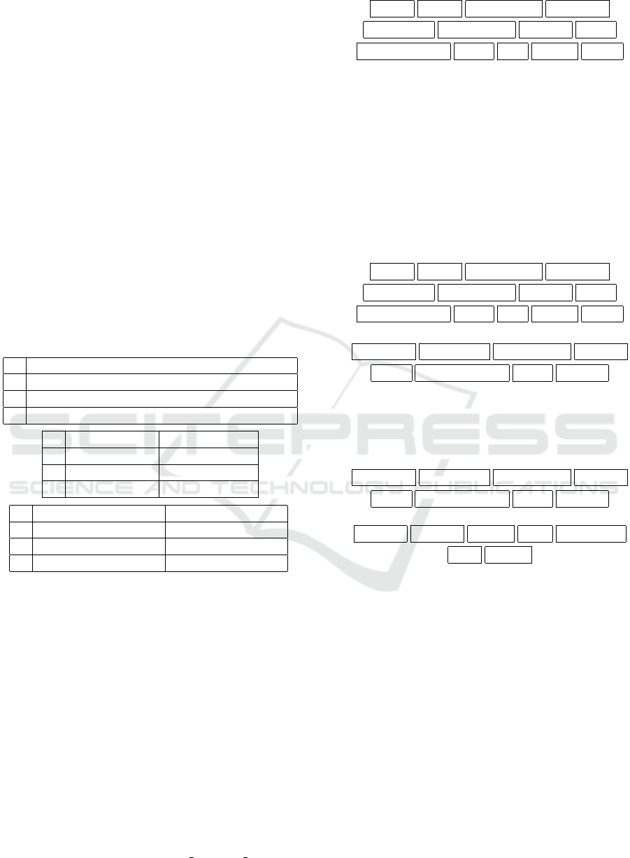
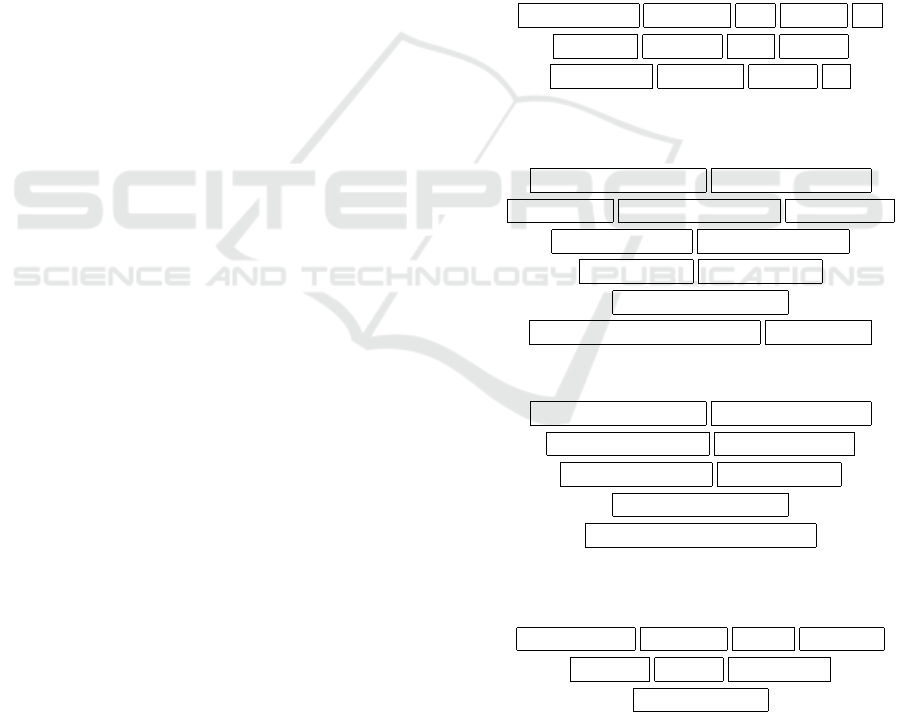
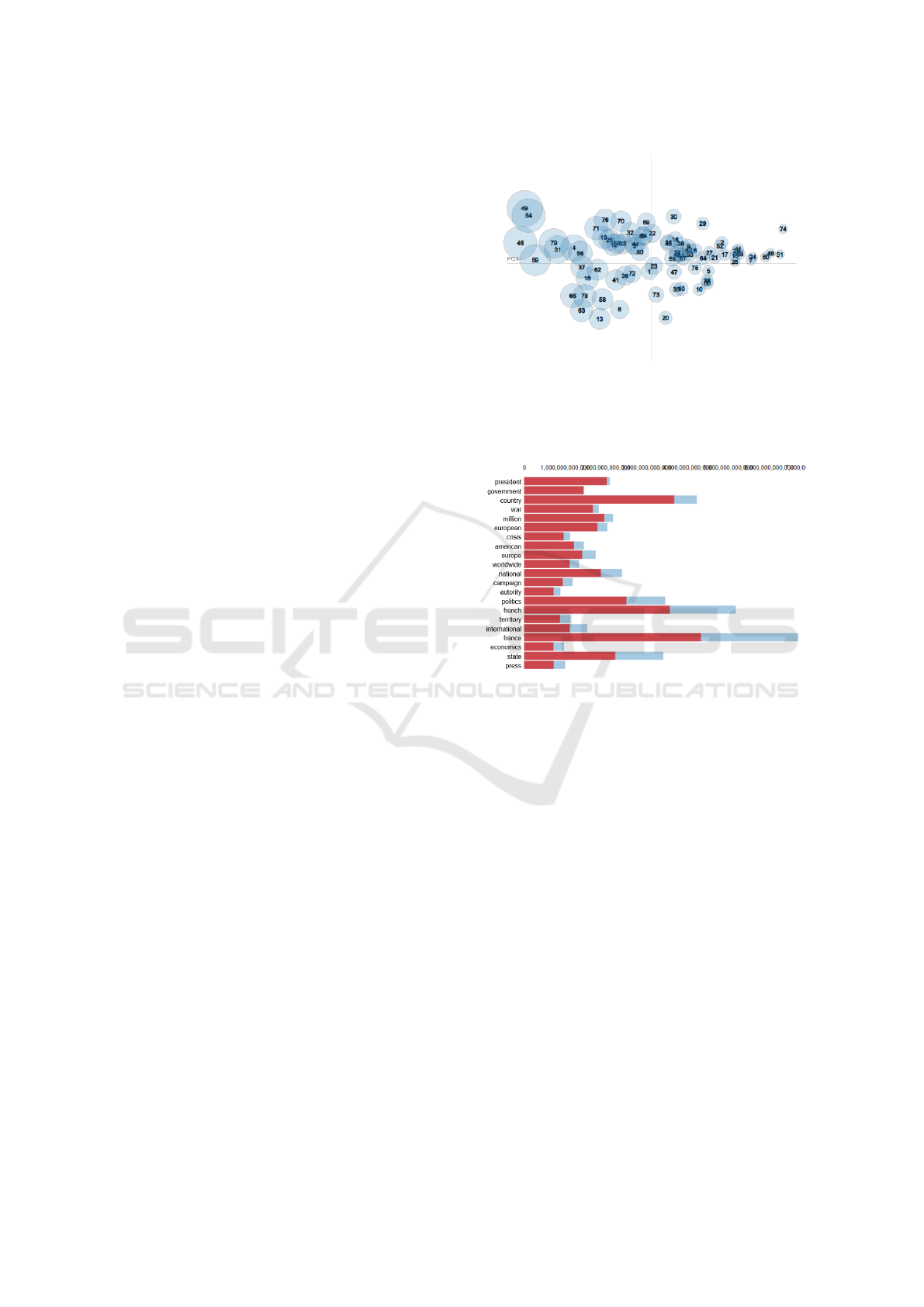
can analyse the topics among themselves (Figure 1)

and their composition (Figure 2).

From these results, we can average probabilities of

words which are on a web page to get the distribution

of topics on the web page (Table 3).

It is essential to note that topic models don’t give

any guarantee on the interpretability of topics created.

Figure 1: PyLDAvis animation with the distribution of top-

ics created with Principal Component Analysis. The more

the point is big, the more the topic is frequent in the corpus

of web pages. Two points nearby on the graph means that

their vocabulary is close.

Figure 2: PyLDAvis animation with the list of words (trans-

lated into English) in a topic example. Red color represents

the frequency of words in the topic, and blue color the fre-

quency of words in all the corpus.

3.2.2 Relevance of the Model

To get the best possible results, we make several tests

of LDA models. We can vary:

• The number of topics expected. The more this

number is high, the more topics are likely to be

precise, but sometimes too speciﬁc. On the con-

trary, a low number of topics will produce general

groups that can contain various subjects in itself.

• The size of the vocabulary. We decide to set min-

imum and maximum thresholds of occurrences in

the vocabulary. Words too occasional or exces-

sively common could affect the model.

We decide to keep default values for other parameters

of LDA model.

To evaluate a LDA model, and in particular choose

the optimal number of topics, we compute some met-

rics. First, perplexity allows to see the behaviour of

the model on unseen data since it is based on a test set

of documents D

test

DATA 2022 - 11th International Conference on Data Science, Technology and Applications

232

Table 3: Example of distribution in n topics created with

LDA on our 3 previous examples.

URL

https://www.doctolib.fr/vaccination-covid-19/paris

https://www.lemonde.fr/actualite-en-continu/

https://www.750g.com/macarons-chocolat-r79291.htm

Topic n°1 Topic n°2 ... Topic n°n

0.32 0.08 ... 0.01

0.00 0.20 ... 0.13

0.67 0.01 ... 0.09

perplexity(D

test

) = exp



−

∑

d=1

log p(w

)

∑

d=1



(6)

M represents the number of documents in the test

set, w

the words in document d and N

the number

of words in document d.

A low score indicates a best performance of gen-

eralisation of the model. However, a known limit is

that optimising for perplexity may not yield human

interpretable topics.

The coherence score in topic modeling is used to

measure how interpretable topics are to humans.

UMass

, w

) = log



D(w

, w

) + 1

D(w

)



(7)

D(w

, w

) indicates how many times words w

and

appear together in documents, D(w

) is how many

time word w

appear alone.

The global coherence of the topic is the average

score on the top N words which describe the topic.

The greater the score is, the better is the coherence.

After trying multiple LDA models with different

parameters, we compare the perplexity and coherence

scores to choose the best model: in our case, it creates

50 topics, and the size of the vocabulary is 1136

words (words must appear on at least 2% of the web

pages of the corpus).

Distribution of probabilities of URL on topics will

be used as features in a model to predict a target,

which is detailed in section 4. It has to be noted that

topics are groups of words that we consider as themes

people can be interested in or not, but here the topics

are not always interpretable for humans.

Figure 3: Examples of words (translated into English) form-

ing topics quite easily interpretable by humans.

Figure 4: Words (translated into English) forming a topic

hard to interpret.

4 IMPACT OF THE ADDITION OF

THESE FEATURES

In this section, we propose to learn a model on the

created features to observe their impact in applica-

tion. The considered target of the model is the socio-

demographic category Woman aged between 25 and

49 years old. Target value is 1 if the panelist is part of

the category, 0 otherwise.

4.1 Input Data Creation

First, we decide to limit the perimeter to 7 days of

web navigation of panelists, which represents roughly

2 million logs (with nearly 400000 belonging to the

target).

Since the target is user-wise, we need to summarise

each panelist’s surf on the period in order to get a

unique value for every feature. The rule chosen de-

pends on the feature’s type:

• Domain and keyword presence dummies as

well as URL clusters are transformed as a per-

cent of logs by user.

• Word clusters and Topics on content are aver-

aged by user.

After this aggregation, we have 459 features for a

User Proﬁling: On the Road from URLs to Semantic Features

233

total of 8993 rows as the number of users (1829 in tar-

get). On table 4 you shall ﬁnd the number of features

for each group.

Table 4: Number of features per group.

Group Features #

G1 Domain and keyword features 96

G2 Topic cluster features 152

G3 Word rarity cluster features 161

G4 Content features 50

TOTAL 459

The data is split in two sets to learn the models on

80% of the panelists and test them on the remaining

20%. This division is made with a draw by stratiﬁca-

tion according to the target.

4.2 Modeling

We decide to run several models, each one consider-

ing one or several groups of the features created in

order to evaluate the impact of each group. Table 5

summarises the features used for each model.

For each model we make a feature selection with

Random Forest Feature Importance. For compari-

son purposes, we set to 100 the number of features

to keep. The single exception comes in Model 1, in

which only the 96 features from G1 are taken into ac-

count, and therefore no feature selection is applied.

The number of features selected per group can be ob-

served in table 6.

Table 5: Groups of features considered in each model.

Model

Group of features

G1 G2 G3 G4

M1 ×

M2 × ×

M3 × ×

M4 × ×

M5 × × × ×

Table 6: Number of features selected in each model.

Group

# of features selected in model

M1 M2 M3 M4 M5

G1 96 25 37 50 16

G2 0 75 0 0 41

G3 0 0 63 0 20

G4 0 0 0 50 23

TOTAL 96 100 100 100 100

The classiﬁer used is a Random Forest and some

basic parameters are tuned, namely the number of

trees, the depth of the trees and the maximum number

of features selected in each node. The model is then

ﬁtted on the train set, and outputs the probability for

each user in the test set to be in the target. Finally, we

proceed to computing precisions and recalls for every

probability threshold and compare the precisions as-

sociated to 3 recall benchmarks of each model. These

are summarised in table 7.

Table 7: Precisions for each model.

Recall

0.1 0.25 0.4

M1 0.385 0.368 0.268

M2 0.474 0.395 0.331

M3 0.468 0.405 0.342

M4 0.42 0.362 0.315

M5 0.544 0.434 0.346

4.3 Results Analysis

Model 1, which is the worst performing model over-

all, was intended to set a benchmark for comparison

purposes with the following models, so no big sur-

prises there.

Models 2 and 3 correspond to the models with fea-

tures created from the raw URL (in addition to the

domain and keyword features). These 2 models yield

close results, but Model 3 has a higher proportion

of features selected coming from the keywords and

domains. The features from group G1 being more

general, they complement probably better the clus-

ters created through TFIDF and NMF, which are more

speciﬁc.

Regarding content features used in Model 4, even

if they seem precise because based on the web pages,

we saw that the process was not practicable on every

URL. In particular, if the period considered is distant

from the moment data is scraped, many URL have

disappeared or their content is empty. The fact that

almost 70% of the logs have ﬁnally no distribution in

topics is a signiﬁcant limit.

At last, Model 5 takes the best each group has to

offer and performs the best with a fairly large margin.

Overall, it improves the results by 30 to 40% depend-

ing on the recall threshold.

5 CONCLUSIONS

In this paper we reviewed different ways to exploit

URLs with the goal of creating meaningful features.

Some are more general than others, but as we have

seen, every group has its share of important, discrimi-

native features. Although the current results speak for

themselves, one might argue we should test the fea-

DATA 2022 - 11th International Conference on Data Science, Technology and Applications

234

tures with other classiﬁers and targets to make further

conclusions.

However, an improvement we could consider is

the use of the time spent on the web page, which is a

notion we have. A user could be weighted in a spe-

ciﬁc topic if they have spent more time on web pages

deeply associated to this topic. Moreover, we solely

focused on the URLs and their content in this paper,

but it should be noted that these features can be part

of a bigger project in which other information is used

in the feature engineering step, like the timestamps,

or the device used, which were not discussed here.

REFERENCES

Chen, E. (2011). Introduction to Latent Dirichlet Alloca-

tion. http://blog.echen.me/2011/08/22/introduction-

to-latent-dirichlet-allocation/.

David M. Blei, Andrew Y. Ng, M. I. J. (2003). Latent

Dirichlet Allocation. Journal of Machine Learning

Research 3.

McCormick, C. (2016). Word2Vec Tutorial - The Skip-

Gram Model. http://mccormickml.com/2016/04/

19/word2vec-tutorial-the-skip-gram-model/.

Mitchell, R. (2015). Web Scraping with Python.

Olivier Grisel, Lars Buitinck, C.-K. Y. (2017). Topic ex-

traction with Non-negative Matrix Factorization and

Latent Dirichlet Allocation. https://scikit-learn.org/st

able/auto examples/applications/plot topics extractio

n with nmf lda.html.

Prabhakaran, S. (2018). LDA in Python – How to grid

search best topic models? https://www.machinel

earningplus.com/nlp/topic-modeling-python-sklearn-

examples/#13compareldamodelperformancescores.

User Proﬁling: On the Road from URLs to Semantic Features

235