
Biodegradation Prediction and Modelling for Decision Support
David F. Nettleton
1a
, Cristina Fernandez-Avila
1b
, Sara Sánchez-Esteva
1
, Steven Verstichel
2c
,
Maria Beatrice Coltelli
3d
, Helena Marti-Soler
1e
, Laura Aliotta
3f
and Vito Gigante
3g
1
IRIS Technology Solutions, Ctra. d'Esplugues, 39-41, 08940 Cornellà de Llobregat, Barcelona, Spain
2
OWS, Dok-Noord 5, 9000 Gent, Belgium
3
Dipartimento di Ingegneria Civile ed Industriale, Università di Pisa, Largo Lucio Lazzarino 56122 Pisa PI, Italy
{laura.aliotta, vito.gigante}@dici.unipi.it
Keywords: Modelling, Simulation, Interpolation, Multi-agent System, Case based Reasoning, Time-Series,
Biodegradation, Bioplastics.
Abstract: In this paper we describe the functionality of a decision support modelling approach to select appropriate
biomaterial blends depending on their mechanical/chemical properties on the one hand, and their
biodegradation behaviour, on the other. Firstly, a Case Based Reasoning (CBR) approach is applied to predict
expected biodegradation behaviour over time, based on historical examples and using a weighted distance
metric on the material properties in order to calculate the trend curve of the new case. Secondly, a Multi-
Agent System (MAS) is applied to dynamically simulate the biodegradation curve, in which the two main
agents, bacteria and plastic, interact to reproduce the biodegradation kinetics over time. The results of the
interpolation are very promising with a good approximation to the real curve time series and % biodegradation,
and the Multi-Agent System successfully simulates the different trend curves over time. The system has been
confirmed as useful by materials expert end-users, who participated in the project, in order to evaluate a priori
new blends “in silico”, and identify and select the most promising, before conducting the long duration
biodegradation experiments in the real environment.
1 INTRODUCTION
Developing biodegradable materials which are fit for
purpose in the future circular economy is a critical
task if we wish to make the transition from fossil fuel
plastics. However, finding an equilibrium between
mechanical properties of the different potential bio-
material blends and their biodegradation
requirements can be a complex, trial and error, and
lengthy process (due to the long experimental time
required for biodegradation testing).
Hence, it is of great interest to be able to
accurately model and predict the biodegradation
process of potential material blends, in order to focus
on the most promising and reduce experimental
a
https://orcid.org/0000-0002-5852-7716
b
https://orcid.org/0000-0002-2678-4347
c
https://orcid.org/0000-0002-4581-6084
d
https://orcid.org/0000-0002-0418-8974
e
https://orcid.org/0000-0002-7127-205X
f
https://orcid.org/0000-0003-1876-5995
g
https://orcid.org/0000-0003-3896-9629
testing time.
In this paper, we show that Case Based Reasoning
and Multi-Agent System modelling approaches can
be useful to generate the biodegradation prediction of
a new blend based on material properties, and
simulate the corresponding biodegradation curve.
The results are very promising, although on a limited
set of cases, for predicting best and worst performers.
First, the CBR obtains the closest historical cases
to a new one, interpolates and expected trend curve,
and then passes this information to the MAS to
simulate in a kinetic and stochastic solution space.
The motivation of using CBR and MAS for
predicting and simulating the biodegradation process,
comes from the shortcomings of existing approaches,
26
Nettleton, D., Fernandez-Avila, C., Sánchez-Esteva, S., Verstichel, S., Coltelli, M., Marti-Soler, H., Aliotta, L. and Gigante, V.
Biodegradation Prediction and Modelling for Decision Suppor t.
DOI: 10.5220/0011136200003274
In Proceedings of the 12th International Conference on Simulation and Modeling Methodologies, Technologies and Applications (SIMULTECH 2022), pages 26-35
ISBN: 978-989-758-578-4; ISSN: 2184-2841
Copyright
c
2022 by SCITEPRESS – Science and Technology Publications, Lda. All rights reserved

such as the need for complex representations of large
amounts of low level chemical knowledge, and the
lack of representation of stochastic and kinetic
features.
The system is defined “as a service”, where
material designers and testers provide the material
characteristics and the system returns the predicted
biodegradation behaviour (curve over time).
The paper is organized as follows: in Section 2
related work is presented, in Section 3 the data used
and pre-processing is summarized, in Section 4 the
Case Based Reasoning processing and matching
approach is described with examples, in Section 5 the
Multi-Agent System based simulation is described
and Section 6 summarizes the work. Also, a Dynamic
System Model definition of the biodegradation
process is given in the Annex.
2 RELATED WORK AND
BACKGROUND
There is an extensive literature of chemical based
biodegradation modelling, using traditional statistical
techniques together with detailed chemical
knowledge (Pavan and Worth, 2006;2008), as well as
more recent approaches based on kinetic
modelling(Farzi et al., 2019; Sonwani et al., 2020;
Sable et al., 2019). However, data modelling using a
simple set of descriptive parameters including
chemical and mechanical properties and using
artificial intelligence techniques is more difficult to
find in the literature. Hence, this is one of the key
motivations and advantages for our current work.
Purely chemical based approaches for the
biodegradability of material require highly
specialized parameterisations, such as in (Alalayah,
2017) (Dragomir et al, 2021), which require deep
chemical knowledge.
Furthermore, sets of ordinary differential
equations (ODEs) have limitations when representing
problems which involve spatial interactions or
emerging properties (Borshchev and Filippov, 2004),
and present difficulties for embodying emergent and
stochastic behaviour. (Pavan and Worth, 2006;2008)
consider QSAR (Quantitative Structure-Activity
Relationship) which is an important family of models
for chemical modelling. QSARs are mathematical
models that can be used to predict different properties
of compounds from the knowledge of their chemical
structure.
In terms of AI techniques applied specifically to
biodegradation modelling, neural networks and rule
induction are two examples. (Gamberger, et al., 1996)
used a rule induction technique and chemical feature
sets as inputs. The biodegradation data from both
data-bases are discrete values, i.e. those chemicals are
classified as biodegradable or non-biodegradable.
The work of (Baker et al., 2004), uses rule induction
and as input includes complex low level chemical
information. Binary output variables are assigned to
each chemical with a 1 for fast biodegradability and 0
for slow biodegradability. (Arranz, et al., 2008) used
neural networks to model biodegradation processes,
requiring a high number of samples to train the
network. Note that in the case of (Gamberger et al.,
1996) and (Baker et al., 2004), their models are
limited to producing a binary classification as output.
In contrast, our solution produces the trend curve with
quantified values for % biodegradation and time.
In their review paper, (Baker et al., 2004)
indicated the use of multiple linear regression and
artificial neural networks, Partial least squares
discriminant analysis and Inductive machine learning
(rule based), among others, however the focus was on
a lower level chemical analysis. Also from (Baker et
al., 2004), a Knowledge-based learning system was
described as a method using machine learning
techniques to determine relevant descriptors
mathematically from data on activity and basic
chemical structure. Furthermore, Multi-Agent based
systems (MAS) (Ferber and Weiss, 1999) and
Dynamic System Models (DSM) (Radzicki and
Taylor, 2008) have been used for stochastic system
modelling in different fields. As recent examples,
(Nettleton et al., 2020) and (Estivill-Castro et al.,
2021) have applied and contrasted the utility of MAS
and DSM for clinical applications, simulating
multiple trend curves over time for modelling
complex kinetic interactions and behaviours between
the human immune system and cancer cells.
The case for using MAS in preference to
mathematical models and DSMs is supported by the
ability of the former to more easily simulate kinetic
and stochastic behaviour, as well as being data driven
so requiring less theoretical know-how to be pre-
defined.
The current work takes (Nettleton et al., 2020) and
(Estivill-Castro et al., 2021) as starting point to apply
the MAS approach to the novel application of
bioplastic blend biodegradation over time. Case
Based Reasoning (CBR) (Aamodt and Plaza, 1994) is
also an approach taken from artificial intelligence
which essentially uses a set of historical cases as a
reference in order to find the closest match to a new
case. In the current work we use CBR as pre-
processing for the MAS, in order to match the
material properties of a new blend to find the closest
Biodegradation Prediction and Modelling for Decision Support
27
historical blends, and hence their corresponding
biodegradation trend curves.
The EU Horizon 2020 project Biontop, of which
the current work forms a part, is aimed at developing
novel packaging films and textiles with tailored end
of life and performance based on bio-based polymers.
In the framework of the project bioplastics blends
based on biobased and industrially compostable
Poly(lactic acid) (PLA) were considered (Narancic et
al., 2018). The blending with other bio-polyesters
resulted successful for modulating the mechanical
properties of this polymer in a wide range of values
(Aliotta et al., 2021;2021). One key aim of the project
is to find bioplastics which are ‘home-compostable’,
which means they are biodegradable at a lower
temperature and in milder conditions than those
typical of ‘industrial composting’.
Hence, the biodegradation testing of blends was
performed for home-composting conditions,
executed according to ISO 14855 but at ambient
temperature (28°C). The tests were carried out using
pellets produced by twin screw extrusion in a Comac
EBC 25 HT extruder (Comac, Milan, Italy).
In the Appendix can be found a dynamic system
model (DSM) simplified representation of the
bioreactor set-up. A DSM typically consists of a stock
and flow diagram (Figure 7), a set of differential
equations to represent the behaviour of the stocks
over time (Table 6), a set of algebraic equations to
define the flows (Table 7), and a set of control
parameters used by the system (Table 8). In Figure 7,
five stocks are defined: bioplastic, compost, Reactor,
O
2
and CO
2
. The flow on the top right indicates the
bioplastic formulation (blend) which is input at the
process start as a batch. The flows below are O
2
which
oxygenated the Reactor and compost, which is input
at the process start as a batch and is the source of the
bacteria. On the right is the CO
2
stock produced as
output (by the biodegradation process) inside the
Reactor stock which is located in the middle. The
degree is biodegradation is quantified from the CO
2
readings.
3 DATA AND PRE-PROCESSING
The data used for prediction and modelling is based
on the materials properties (chemical and
mechanical) as shown in Table 1, and the
biodegradation results of each material, as shown in
Table 2 and Figures 1 and 2. Eight material blends
were used for biodegradation testing, as part of the
Biontop project (see background Section). Note that
for confidentiality reasons and intellectual property
protection of the Biontop project, the data has been
normalized or rescaled, and the material names
anonymized. However, this has been done in a way
so as to maintain the relative values and
interpretability of the data with the results.
Table 1 shows a summary of the chemical and
mechanical properties of the eight main bioplastic
materials, named as blends 1 to 8. For confidentiality
reasons, all material property values are normalized
in a range between 0.5 and 1.5, and the
biodegradation times are scaled between 0 and 1. It
can be seen that in terms of chemical properties, blend
7 has a low molecular weight and medium polarity
and crystallinity; in terms of mechanical properties, it
has a low Young’s Modulus, a low elongation at
break and a high tensile strength.
Table 2 shows a summary of the biodegradation
results for the eight material blends whose
characteristics were given in Table 1. It can be seen
that blend 7 gives the best biodegradation results,
reaching 100% biodegradation in a scaled time of 0.6.
On the other extreme, the blend 5 material gives the
worst biodegradation results, achieving only 1.2%
biodegradation in a scaled time of 1.0 (highest value).
From the material characteristics of Table 1 and
the biodegradation results of Table 2, a strong
correlation is evident between the two. For example,
a low molecular weight and high crystallinity give a
propensity for the material to biodegrade.
We note that only eight cases (i.e. blends) were
available from the Biontop project with their full
material properties data and biodegradation results.
However, they were chosen, by the materials experts
involved in the project, to cover a realistic and
representative distribution of scenarios from good
biodegradation (blends 4 and 6 to 8), medium (blend
3) and poor (blends 1, 2 and 5).
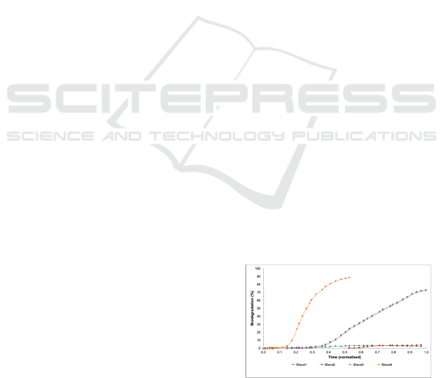
Figures 1 and 2 show all the biodegradation trend
curves for the eight blends which were empirically
tested.
Figure 1: Biodegradation curves for blends 1 to 4.
SIMULTECH 2022 - 12th International Conference on Simulation and Modeling Methodologies, Technologies and Applications
28
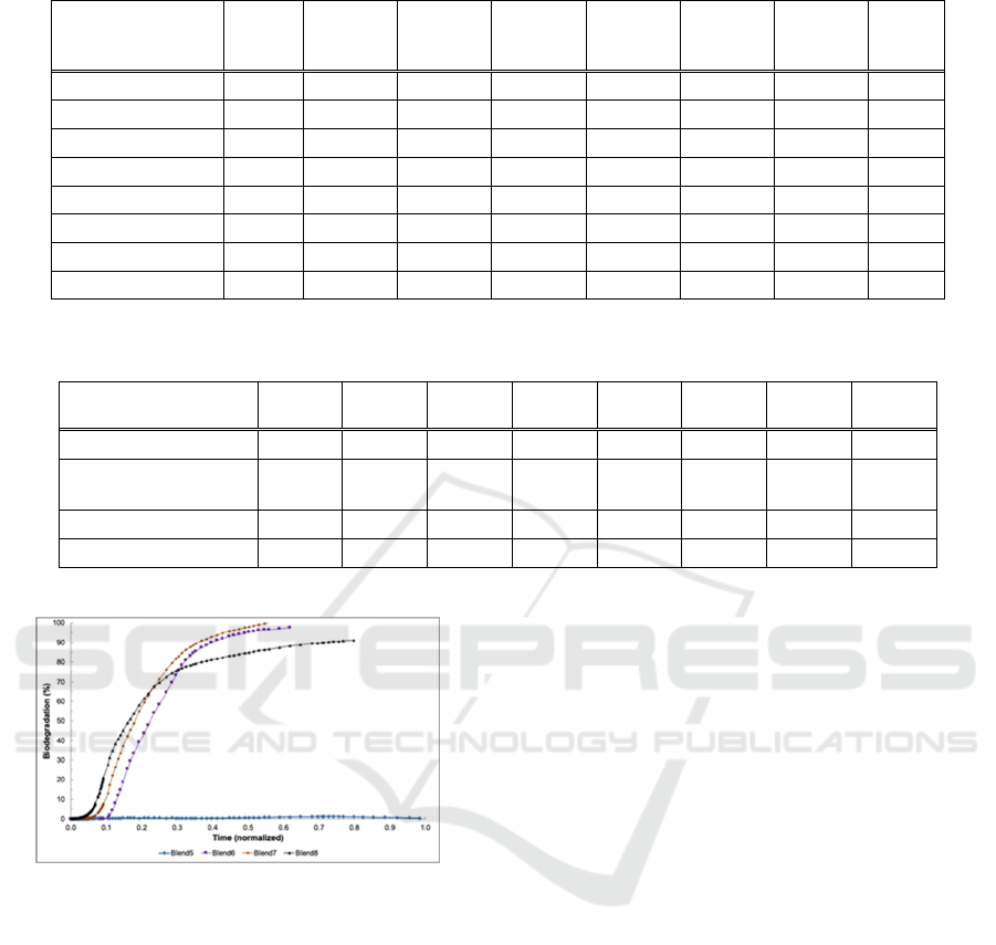
Table 1: Chemical and mechanical properties of blends 1 to 8*.
Chemical and
Mechanical
Properties
Blend1 Blend2 Blend3 Blend4 Blend5 Blend6 Blend7 Blend8
Polarity 0.7 0.7 1.4 1.5 0.8 1.3 1.2 1.1
Molecular weights 1.5 1.4 0.9 0.7 1.3 0.6 0.6 0.5
Crystallinity 1.5 1.2 0.9 0.7 1.5 0.7 0.8 0.5
MFR 0.5 0.6 0.6 0.7 1.3 1.4 1.4 1.5
Impact strength 0.7 0.8 0.9 1.5 0.7 1.4 1.4 1.5
Tensile strength 1.2 1.1 0.5 0.9 1.5 0.5 0.6 0.8
Young's Modulus 1.5 1.3 1.0 0.8 1.5 0.5 0.5 0.6
Elongation at break 0.5 0.7 1.1 1.5 0.5 1.2 1.2 1.2
*All values are normalized to a range between 0.5 and 1.5.
Table 2: Biodegradation results of blends 1 to 8*.
Biodegradation
Criteria
Blend1 Blend2 Blend3 Blend4 Blend5 Blend6 Blend7
Blend8
Time to 50% 0.8 0.3 0.2 0.2 0.2
Time to 100% or
MAX
0.6 1.0 1.0 0.5 1.0 0.6 0.6 0.7
Max% 3.5 4.2 73 88 1.2 97.7 100 90.3
Rank biodegradability 6 7 5 4 8 2 1 3
*All values (except max%) are scaled to a range between 0 and 1.0.
Figure 2: Biodegradation curves for blends 5 to 8.
4 CASE BASED MATCHING
In this section we explain how the Case Based
Matching approach with an appropriate distance
metric, is applied to the material properties and
biodegradation data in order to predict the
biodegradation of new blends.
4.1 Modus Operandi and Example
Applying CBM to Material
Properties and Blend
Biodegradation Data
The data processing of the CBM approach has the
following four steps, with reference to Table 3, Figure
3 and Equation (1): (i) choose one blend as “new
blend” (e.g. blend8); (ii) calculate “distance” between
new blend and all remaining historical blends using
only material properties data (i.e. only a priori
information); (iii) identify two “closest” historical
blends in terms of distance (e.g. blends 6 and 7); (iv)
use the two “closest” historical blends to interpolate
curve of “new blend” (Figure 3).
The distance D is calculated by applying a
Euclidean metric to the respective material properties
(Table 1) and summing over n, the number of
properties, which are previously normalized and have
equal weighting:
D
∑
|𝑝
𝑝
|
(1)
where 𝑝
is property i of material 1 and 𝑝
is
property i of material 2.
Table 3 shows the seven blends used as the
historical case base and blend 8 considered as a “new”
blend (but whose biodegradation results are known).
Blends 6 and 7 are found to be the “closest” to blend
8 (from all 7 available historical blends) using the
distance metric calculation. This gives a distance of
0.7 and 0.6, respectively for blends 6 and 7.
Biodegradation Prediction and Modelling for Decision Support
29
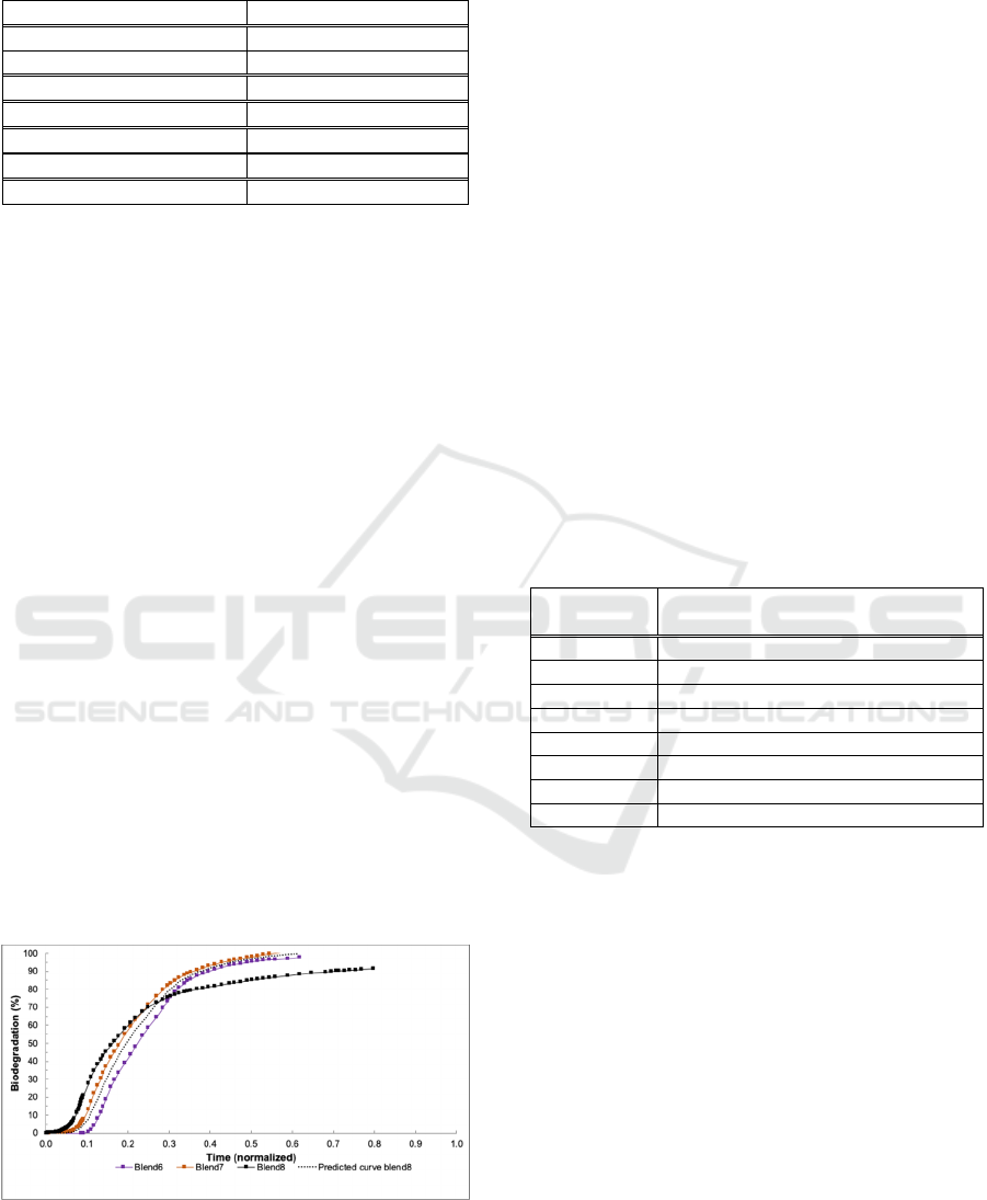
Table 3: Blends selected as historical examples and new
blend.
Historical examples Distance to Blend 8
Blend1 1.5
Blend2 1.5
Blend3 1.0
Blend4 0.8
Blend5 1.5
Blend6 0.7
Blend7 0.6
Now, using the curve points 𝑦
and 𝑦
of existing
blends 6 and 7, respectively, the corresponding curve
point approximation 𝑦
for the new blend is obtained:
first the distances of Table 3 are normalized and then
the two smallest values used as weights
𝑤
and 𝑤
to
interpolate. From this, the polynomial equation is
estimated which best fits the curves 𝑌
and 𝑌
and the
individual points 𝑦
(% biodegradation over time)
are calculated thus:
∀𝑦 0, 𝑤∈
0. .1
𝑦′
𝑦
𝑤
(2)
𝑦′
𝑦
𝑤
𝑦
𝑦′
𝑦′
Hence, the overall result of the case matching of a
new blend with historical blends, is to obtain a new
interpolated biodegradation trend curve over time. In
Figure 3 it is shown that blends 6 and 7 are identified
as the closest blends to the “new” blend 8, based on
chemical and mechanical properties. Also in Figure 3
is seen how the blend 8 curve is interpolated from the
curves of blends 6 and 7, using the weighted distance
metric (Equation 2) to generate the points. In the case
of blend 8, the fit of the interpolated curve to the real
blend 8 curve is relatively lower (0.75, see Table 4).
Figure 3: Closest historical curves and new curve
interpolation.
This is because the trend of the real curve for blend 8
flattens out from time 0.3 onwards, diverging from
the trends of blend curves 6 and 7. However, at this
point it has already reached almost 80%
biodegradation (Figure 2).
4.2 Results of Applying CBM to Predict
Biodegradation Curve of Blends
The process described in Section 4.1 with blend 8 as
the “new blend”, was repeated for blends 1 to 7. Table
4 shows the results of comparing the trend curves
predicted by CBM with the real curves, for each of
the blends. It can be seen that all the R
2
values of the
matches were over 0.81, with the exception of blends
3 and 8, with R
2
values of 0.68 and 0.75, respectively.
The lower performance for blends 3 and 8 was
expected as they have intermediate biodegradation
performance with respect to the best blends for
biodegradation and the worst ones (see Figures 1 and
2). In summary, estimated blend curves 1, 2 and 5 are
fitting closely together, also blends 4, 6 and 7, while
blends 3 and 8 are relative ‘outliers’. This is
supported by the R
2`
values shown in Table 4.
Table 4: Matching of simulated data trend curve (simulated
data) with real trend curve - R
2
value.
Composition
/Blen
d
Trend curve (simulated data) vs trend
curve (real data)
–
R
2
value
Blend1 0.9440
Blend2 0.9379
Blend3 0.6830
Blend4 0.8174
Blend5 0.9373
Blend6 0.9002
Blend7 0.8907
Blend8 0.7506
Furthermore, two aspects are of interest to the
material experts: what is the % degradation at time
0.6 (or less) and how long does it take to reach a given
biodegradation %. In general, the estimated curves
provide a good approximation of this information.
Note that for blends 3 and 8, the matching is with
curves of shorter duration (0.6) and so the estimated
curves get truncated at this limit. Hence, in
conclusion, special attention has to be made to
defining similar experimental conditions (time
duration) for blend testing and having sub-groups of
similar blends for comparison proximity. The
accuracy for % at time 0.6 was generally within 15%
for blends 3 and 8, 10% for blends 4, 6 and 7, and
within 5% for blends 1,2 and 5. For the former, this
was more dependent on the cut-off time of the closest
blends chosen.
SIMULTECH 2022 - 12th International Conference on Simulation and Modeling Methodologies, Technologies and Applications
30

5 MULTI-AGENT SIMULATION
In this section we use a Multi-Agent System (MAS)
to simulate the blend biodegradation behaviour, based
on the trend curves. This requires the adjustment of
the MAS control parameters (biodegrade chance,
biodegrade distance, detect distance, speed) which act
in a 2D solution space during the process.
As a starting point, the control parameters are
assigned as a generic “predator-prey” model (Bădică
et al., 2018; Karsai et al., 2016) which is interpreted
in the current context as a kinetic model where the
predator is the bacteria and the prey is the plastic.
Furthermore, a plastic agent remains fairly static
whereas a bacterium is more mobile, performing a
random walk at a given “speed” (SP) until a plastic
agent comes within its “detect distance” (DD). Once
this happens the bacteria agent moves directly
towards the plastic agent until it reaches the
“biodegrade distance” (BD), and then, depending on
the “biodegrade chance” (BC), it will biodegrade the
plastic agent (i.e. the plastic agent is consumed and
disappears). This apparently simple individual
behaviour can give rise to a complex collective
system, and more advanced interaction rules can be
programmed into the agents. Figure 4 illustrates the
concept of the two dimensional state space and
respective action distances between the agents.
Figure 4: State space definition for agent interactions.
5.1 Modus Operandi
It is recalled that the CBM processing approach
applied in Section 4 obtains the polynomial trend
curve for the new blend. Now, we provide the trend
curve (polynomial equation) to the MAS, and as it
runs the agent system control parameters adapt in
order to keep the population (of plastic) as close as
possible to the trend curve. A weighting is also used
for each control parameter.
The process is repeated ad-hoc for several trend
curves, until a historical of results (trend curves with
their corresponding agent control parameters) is
accumulated. Once sufficient historical examples are
available, the agent control parameter initial values
and weighting can be automatically estimated for a
new trend curve, without having to perform ad-hoc
testing (thus significantly reducing the testing and
refinement cycles to obtain the settings).
The control parameters are updated as follows: let
P
1
be the expected plastic biodegradation percentage
calculated from the trend curve and P
2
the current
plastic agent population percentage in the MAS.
Then, the percentage difference 𝑃
∆
between the two
will be:
𝑃
∆
.
Next, a multiplier coefficient is defined as:
𝑚𝑢 1.0 𝑃
∆
Then, the update rules are defined as:
𝐵𝐶 𝑚𝑖𝑛
1, 𝐵𝐶 𝑚𝑢
𝐵𝐷 𝐵𝐷 𝑚𝑖𝑛
1, 𝑚𝑢
𝑆𝑃 𝑆𝑃 𝑚𝑢
𝐷𝐷 𝐷𝐷 𝑚𝑢 (3)
where BC = biodegrade chance, BD = biodegrade
distance, SP = speed and DD = detect distance.
5.2 Results of Applying MAS to Blend
Biodegradation Data
Figure 5 shows the results for the agent simulation
processing the blend 3 trend curve. On the left are the
Multi-Agent user interface screens where the blue
dots represent the “plastic agents” and the green dots
represent the “bacteria agents”. The initial state is
seen on the top left (with an equal amount of blue and
green dots) and the final state is on the bottom left
(with many more green and less blue). That is, the
biodegradation process has worked, the bacteria have
biodegraded the plastic. The right side of Figure 5
shows the corresponding simulation over time
(accelerated time which processes a long time period
in just a few minutes). On the top right is the real
biodegradation curve for the new blend 3, and on the
bottom right (green line) is the Multi-Agent
simulation result. It can be seen that the simulated
curve (bottom right) is a good approximation of the
real curve (top right) in final percentage reached
(70%) and normalized time duration of 1.0, as well as
the gradient and general trend of the curve.
Biodegradation Prediction and Modelling for Decision Support
31
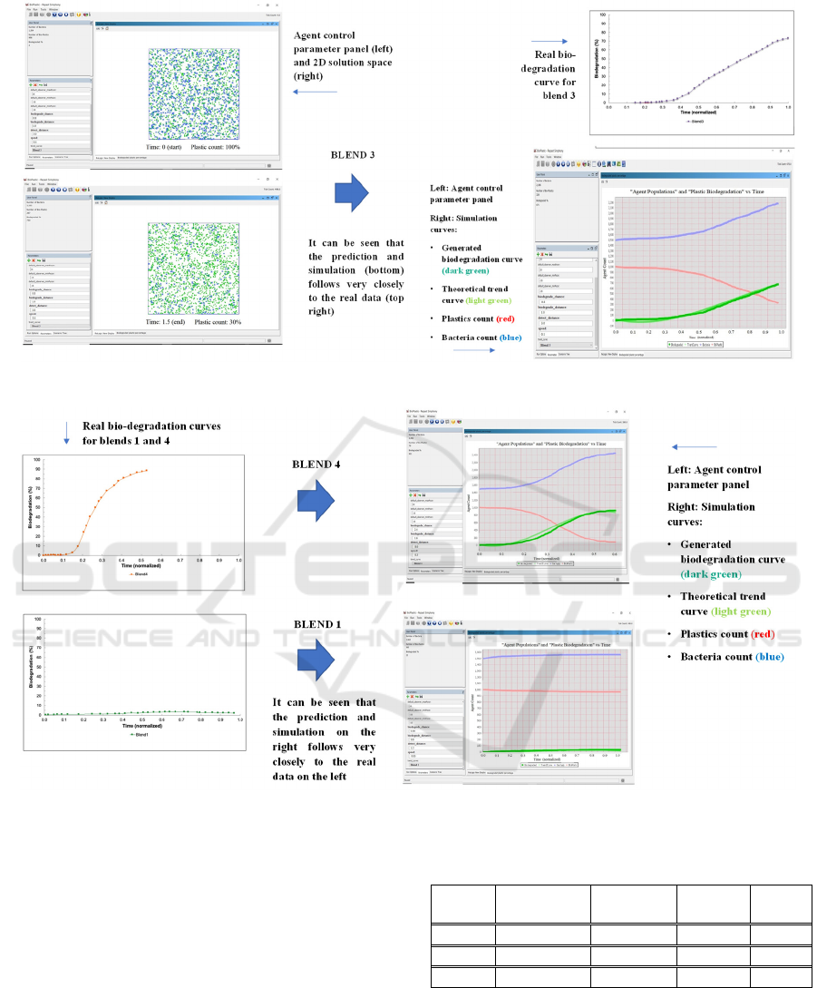
Figure 5: Agent simulation (Blend 3).
Figure 6: Agent simulation (Blends 1 and 4).
Having successfully simulated blend 3, we now
perform the same process for blends 1 and 4, as
shown in Figure 6. These blends represent the best
performer and the worst, respectively, in terms of
biodegradation behaviour. On the left of Figure 6 are
shown the real trend curves over time, where it can be
seen that blend 4 reaches 90% biodegradation with a
normalized time duration of 0.6, whereas the blend 1
only achieves a max. of 5% with a normalized time
duration of 0.8. On the right of Figure 6 it can be seen
that the Multi-Agent system successfully models both
trend curves over time and % end point, with the
green curve of blend 4 shown on the top right and the
green curve of blend 1 shown on the bottom right.
Table 5: Multi-agent system control parameters for three
different biodegradation simulations*.
Bio-degrade
chance
Bio-degrade
distance
Detect
distance
Speed
Blend 1 0.08 0.8 1.5 0.03
Blend 3 0.8 1.0 3.0 0.1
Blend 4 2.4 1.6 8.0 0.3
*Values have been anonymized while maintaining their relative magnitudes.
Table 5 shows the control parameters used for the
simulations of biodegradation for blends 1, 3 and 4,
which are depicted in Figures 5 and 6. The four
control parameters are given which relate to the
bacteria and plastic agents: distance in which a
bacteria agent can detect and “biodegrade” a plastic
SIMULTECH 2022 - 12th International Conference on Simulation and Modeling Methodologies, Technologies and Applications
32

agent, and the speed of movement for the bacteria
agent.
It can be seen that blend 4, which has one of the
best biodegradation behaviours (in terms of time and
%, see Table 2) has the highest relative values for all
four control parameters. On the other hand, blend 1,
which has the worst biodegradation, has the lowest
values, also for all four control parameters. This is
explained by the degree of “excitation” of the system
necessary in order to replicate the biodegradation
curves (see Figures 5 and 6) in terms of agent
populations. It could be interpreted as a degree of
“kinetic energy” of the bacteria and the plastic. Blend
3, which displays an intermediate level of
biodegradation, shows intermediate values for its
control parameters, relative to blends 1 and 4,
however the relation between the control parameters
of the blends is non-linear. For example, the
“biodegrade chance” for blend 1 is 10 times less than
blend 3, whereas the “biodegrade chance” of blend 4
is only three times that of blend 3. It can be
interpreted also in terms of the “distance” between the
trend curves (Figures 5 and 6) and also between the
respective material properties (Table 1).
In each case, the MAS control parameters have
been optimized manually for each blend. However, as
we progressively obtain a set of historical settings,
they can be used to approximate settings (at least as
an initial starting point) for new blends, in a similar
way to the CBR, based on some distance function
related to the material properties.
6 CONCLUSIONS
In this paper we have explained how a Case Based
Reasoning (CBR) approach can be used to predict a
biodegradation trend curve over time and how a
Multi-Agent System can be applied to simulating the
biodegradation process.
The CBR approach has been demonstrated to be
able to generate a biodegradation prediction and trend
curve for a blend, which is a good fit to real data,
using the chemical/mechanical properties for
matching closest historical cases, which is calculated
using a weighted distance function. The results in
Table 4 show all R
2
fitting values of predicted vs real
curves to be over 0.81, with the exception of outlier
blends 3 and 8 (refer to Section 4.2 for explanation).
Furthermore, we have demonstrated how a MAS
can be used to simulate the corresponding
biodegradation curves, with dynamic weighted MAS
control parameter calculation (Table 5) tuned for each
trend curve.
The results are clearly promising and verified as
useful by the materials experts who design blends
which must comply with given chemical and
mechanical properties on the one hand, and
biodegradation characteristics on the other.
The choice of material properties provided a
strong set of descriptors with a good correlation
between chemical and mechanical properties and
their biodegradation behaviour. However, in order to
obtain a good predictive capability from the CBR, a
combination of a non-trivial weighted distance
calculation and an interpolation method were
necessary. In the case of the MAS, the real-time
control parameter optimization also used a set of non-
trivial updating formulas including weighting factors.
Overall, the approaches appear to offer promising
solutions for a variety of bioplastic blends, for their
biodegradation trend prediction and dynamic
simulation, respectively.
Also, the MAS offers a simulation solution which
is relatively easy to implement and calibrate, in
contrast with DSM and mathematical modelling
approaches. Furthermore, the MAS is able to embody
stochastic and noisy features present in real systems,
As future work, as part of the ongoing Biontop
project, we expect to incorporate new blends into the
modelling. Also, we plan to develop further the MAS
modelling, by improving the induction of the MAS
control parameters from the material properties, thus
generating the trend curve automatically.
Furthermore, the MAS control parameters, which
were initially optimized manually for the different
blends, can be used to find settings for new blends, in
a similar way to the CBR approach.
ACKNOWLEDGEMENTS
The BIONTOP project has received funding from the
Bio Based Industries Joint Undertaking under the
European Union’s Horizon 2020 research and
innovation programme under grant agreement No
837761.
REFERENCES
Aamodt, A., Plaza, E. (1994). "Case-Based Reasoning:
Foundational Issues, Methodological Variations, and
System Approaches," Artificial Intelligence
Communications 7 (1994): 1, 39-52.
Alalayah, W. M. (2017). Simulation of the biodegradation
of petroleum hydrocarbons utilizing Artificial Neural
Networks. International Journal of Engineering
Development and Research, 5(4), 891-896.
Biodegradation Prediction and Modelling for Decision Support
33

Aliotta, L., Vannozzi, A., Canesi, I., Cinelli, P., Coltelli,
M.-B., Lazzeri, A. (2021). Poly(lactic acid)
(PLA)/Poly(butylene succinate-co-adipate) (PBSA)
Compatibilized Binary Biobased Blends: Melt Fluidity,
Morphological, Thermo-Mechanical and Micro-
mechanical Analysis. Polymers 2021, 13, 218.
https://doi.org/10.3390/polym13020218.
Aliotta, L., Gigante, V., Coltelli, M.-B., Lazzeri, A. (2021).
Volume Change during Creep and Micromechanical
Deformation Processes in PLA–PBSA Binary Blends.
Polymers 2021, 13, 2379. https://doi.org/10.3390/
polym13142379.
Arranz, A., Bordel, S., Villaverde, S., Zamarreño, J. M.,
Guieysse, B., & Muñoz, R. (2008). Modeling
photosynthetically oxygenated biodegradation
processes using artificial neural networks. Journal of
hazardous materials, 155(1-2), 51-57.
Bădică, A., Bădică, C., Ivanović, M., & Dănciulescu, D.
(2018). Multi‐agent modelling and simulation of graph‐
based predator–prey dynamic systems: A BDI
approach. Expert Systems, 35(5), e12263.
Baker, J. R., Gamberger, D., Mihelcic, J. R., Sabljić, A.
(2004). Evaluation of Artificial Intelligence Based
Models for Chemical Biodegradability Prediction,
Molecules. 2004 Dec; 9(12): 989–1003.
Borshchev, A. and Filippov, A. (2004). From system
dynamics and discrete event to practical agent based
modeling: Reasons, techniques, tools. 22nd Int. Conf.
of the System Dynamics Society.
Dragomir, T. L., Pană, A. M., Ordodi, V., Gherman, V.,
Dumitrel, G. A., & Nanu, S. (2021). An Empirical
Model for Predicting Biodegradation Profiles of
Glycopolymers. Polymers, 13(11), 1819.
Estivill-Castro, V., Hernández-Jiménez, E., Nettleton, D. F.
(2021). A system dynamics model approach for
simulating hyper-inflammation in different COVID-19
patient scenarios. In 11th International Conference on
Simulation and Modeling Methodologies, Tech-
nologies and Applications, SIMULTECH 2021 (pp.
141-143).
Farzi, A., Dehnad, A., Fotouhi, A. F. (2019).
Biodegradation of polyethylene terephthalate waste
using Streptomyces species and kinetic modeling of the
process. Biocatalysis and agricultural biotechnology,
17, 25-31.
Ferber, J., Weiss, G. (1999). Multi-agent systems: an
introduction to distributed artificial intelligence (Vol.
1). Reading: Addison-Wesley.
Gamberger, D., Sekušak, S., Medven, Ž., & Sabljić, A.
(1996). Application of artificial intelligence in
biodegradation modelling. In Biodegradability
Prediction (pp. 41-50). Springer, Dordrecht.
Karsai, I., Montano, E., and Schmickl, T. (2016). Bottomup
ecology: an agent-based model on the interactions
between competition and predation. Letters in
Biomathematics, 3(1):161–180.
Narancic, T., Verstichel, S., Reddy Chaganti S., Morales-
Gamez, L., Kenny, S.T., De Wilde, B,, Babu Padamati,
R., O'Connor, K. E. (2018). Biodegradable Plastic
Blends Create New Possibilities for End-of-Life
Management of Plastics but They Are Not a Panacea
for Plastic Pollution. Environ Sci Technol. 2018 Sep
18;52(18):10441-10452. doi: 10.1021/acs.est.8b02963.
Epub 2018 Aug 29. PMID: 30156110.
Nettleton, D. F., Estivill-Castro, V., Jiménez, E. H. (2020).
Multi-agent Modeling Simulation of In-vitro T-cells for
Immunologic Alternatives to Cancer Treatment. In
ICAART (1) (pp. 169-178).
Pavan, M., Worth, A. (2006). Review of QSAR Models for
Ready Biodegradation.
Pavan, M., Worth, A.P. (2008). Review of Estimation
Models for Biodegradation, QSAR & Combinatorial
Science, Vol. 27, Issue 1, Special Issue: Computational
Assessment of Toxicity and Environmental Fate,
January 2008, Pages 32-40.
Radzicki, M.J., Taylor, R.A. (2008). Origin of System
Dynamics: Jay W. Forrester and the History of System
Dynamics. In: U.S. Department of Energy's
Introduction to System Dynamics. Retrieved 23
October 2008.
Sable, S., Mandal, D. K., Ahuja, S., & Bhunia, H. (2019).
Biodegradation kinetic modeling of oxo-biodegradable
polypropylene/polylactide/nanoclay blends and
composites under controlled composting conditions.
Journal of environmental management, 249, 109186.
Sonwani, R. K., Swain, G., Giri, B. S., Singh, R. S., Rai, B.
N. (2020). Biodegradation of Congo red dye in a
moving bed biofilm reactor: Performance evaluation
and kinetic modeling. Bioresource Technology, 302,
122811.
APPENDIX
The following defines the Dynamic System Model
representation of the biodegradation process. Figure
7 shows the overall schema of stocks and flows,
Tables 6 and 7 show the differential and algebraic
equations, respectively, and Table 8 shows the
systemic variables and parameters. See Section 2 of
the paper for further explanation.
SIMULTECH 2022 - 12th International Conference on Simulation and Modeling Methodologies, Technologies and Applications
34
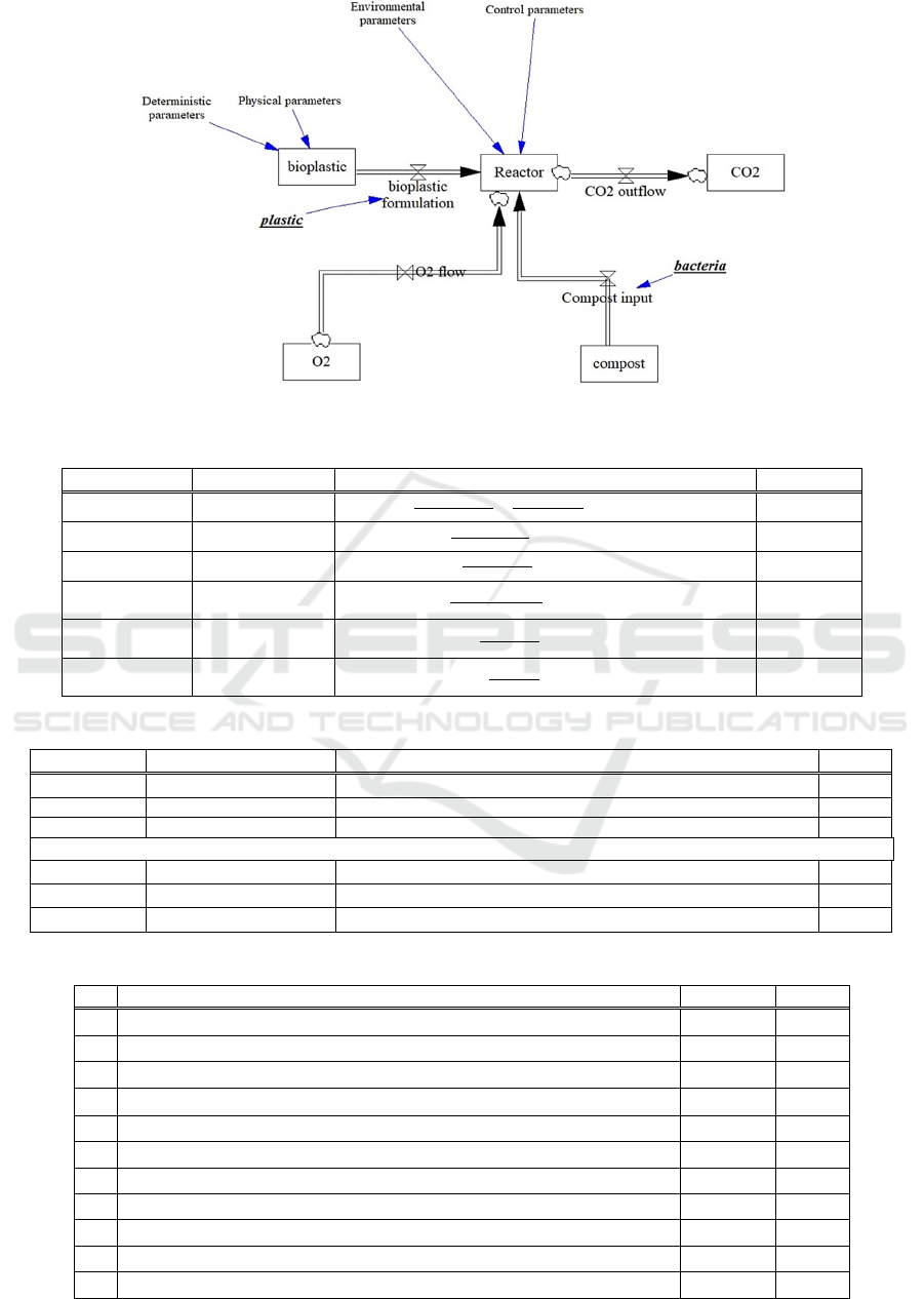
Figure 7: Stocks and Flows.
Table 6: Differential Equations.
Equation no. Stoc
k
Differential equations Units
1 Reactor
𝑟𝑒𝑎𝑐𝑡𝑜𝑟(t)
kg/d
2 Bioplastic
𝑏𝑖𝑜𝑝𝑙𝑎𝑠𝑡𝑖𝑐(t)
kg/d
3 Compost
compost(t)
kg/d
4 Bacteria
𝑑𝑏𝑎𝑐𝑡𝑒𝑟𝑖𝑎𝑡
𝑑𝑡
bacteriat
%
5 CO2
𝑑𝐶𝑂2𝑡
𝑑𝑡
𝐶𝑂2𝑡
cm
3
/h
6 O2
𝑑𝑂2𝑡
𝑑𝑡
𝑂2𝑡
cm
3
/h
Table 7: Algebraic Equations.
Equation no. Flow Algebraic equations Units
1 Biodecomposition material Biodegradation material(t) = bioplastic(t) + compost(t) + O2(t) – CO2(t) kg/h
2 O2 O2(t) = O2 cm
3
/h
3 CO2 CO2(t) = CO2 cm
3
/h
Quality criteria
4
Quality 1 Decomposition time days
5
Quality 2
% decomposition
*
achieved (absolute and/or relative)
%
6
Quality 3
Time to reach a target decomposition
*
days
Table 8: Systemic variables and parameters.
Nº. Paramete
r
Value
(
s
)
Units
1
Amount of bioplastic
c
1
kg
2
Amount of compost
c
2
kg
3
Bioplastic formulation
c
3
-
4
Average absolute humidity
c
4
g/M
3
5
O2
c
5
cm
3
/h
6
CO2
c
6
cm
3
/h
7
Cut off time
c
7
days
8
Cut off %
c
8
%
9
Mechanical properties of bioplastics
p
1
, p
n
10
Chemical properties of bioplastics (DETERMINISTIC)
d
1
,
, d
n
11 Composting conditions (ENVIRONMENTAL, less DETERMINISTIC) e
1
,
, e
n
Biodegradation Prediction and Modelling for Decision Support
35
