Forecast of Dengue Cases based on the Deep Learning Approach:

A Case Study for a Brazilian City

Luiz Sérgio de Souza

, Solange Nice Alves-Souza

, Lucia Vilela Leite Filgueiras

Leandro Manuel Reis Velloso

, Mailson Fontes de Carvalho

, Luciano Anísio Garcia

Marcia Ito

, Johne Marcus Jarske

, Tânia Letícia dos Santos

Henrique Mathias Fernandes

, Gabriela Momberg Araújo

and Wesley Lourenço Barbosa

Faculdade de Tecnologia do Estado de São Paulo (FATEC), Centro Estadual de Educação Tecnológica Paula Souza,

Brazil

Departamento de Engenharia de Computação e Sistemas Digitais (PCS), Universidade de São Paulo (USP), Brazil

Faculdade de Arquitetura e Urbanismo (FAU), Universidade de São Paulo (USP), Brazil

Universidade Federal do Piauí (UFPI), Brazil

Universidade de São Paulo (USP), Programa de Pós-graduação em Sistemas de Informação, Brazil

Universidade de São Paulo (USP), Curso de Biblioteconomia, São Paulo (SP), Brazil

Universidade de São Paulo (USP), Programa de Pós-graduação em Engenharia Elétrica, São Paulo (SP), Brazil

{ssouza. lfilguei, leandrovelloso, luciano.garcia, johne.jarske, fernandeshm1997, wesleyloubar}@usp.br,

gabriela.momberg.araujo@alumni.usp.br, tania.leticia2011@gmail.com, marciaito2000@gmail.com

Keywords: Forecasting, Time Series, Dengue, Deep Learning, LSTM, MLP.

Abstract: According to the World Health Organization (WHO), dengue is an endemic disease in more than 100

countries, with about 50 million people infected each year and 2.5 billion living in risk areas. Dengue requires

a major research effort in countries affected by the disease, as its incidence is strongly determined by non-

linear local processes, such as climatic conditions, social characteristics and habits of populations (Falcón-

Lezama, 2016). In this scenario, forecasting models can be important tools for outbreak control, allowing

health institutions to anticipate the mobilization of resources. In this article, we use deep learning, including

long and short-term memory (LSTM) and dense layers of perceptrons to implement a forecast model of

dengue cases for 5 epidemiological weeks ahead with a mean accuracy of 93%.

1 INTRODUCTION

Predicting the future and based on that, intervening in

current processes is a fundamental task since the

adoption of mechanisms for analyzing and

https://orcid.org/0000-0002-7855-0235

https://orcid.org/0000-0002-6112-3536

https://orcid.org/0000-0003-3791-6269

https://orcid.org/0000-0003-4883-7208

https://orcid.org/0000-0003-0110-7136

https://orcid.org/0000-0001-7163-6987

https://orcid.org/0000-0003-4799-2433

https://orcid.org/0000-0001-8907-6455

https://orcid.org/0000-0001-6912-6793

https://orcid.org/0000-0002-9916-9150

https://orcid.org/0000-0001-9249-8325

https://orcid.org/0000-0001-6106-7936

forecasting health incidents contributes to reducing

expenditure and decreasing the mortality rate and the

number of people affected by the diseases.

Nevertheless, forecasting should not be considered

the final answer, but rather a tool to increase

Sérgio de Souza, L., Alves-Souza, S., Filgueiras, L., Velloso, L., Fontes de Car valho, M., Garcia, L., Ito, M., Jarske, J., Santos, T., Fernandes, H., Araújo, G. and Barbosa, W.

Forecast of Dengue Cases based on the Deep Learning Approach: A Case Study for a Brazilian City.

DOI: 10.5220/0011135500003277

In Proceedings of the 3rd International Conference on Deep Lear ning Theory and Applications (DeLTA 2022), pages 71-76

ISBN: 978-989-758-584-5; ISSN: 2184-9277

understanding and highlight important processes and

guide action (De la Sante, 1999).

Machine Learning (ML) is data-driven and does

not involve intense prior assumptions, enabling the

mapping of non-linear functions, even if the

relationships between the data are not known (Wang

et al., 2015). According to Cortes et al (2018), in the

last decades, non-linear models of automatic learning

have attracted the attention of researchers because

they present good performance for forecasting non-

stationary time series when compared with models of

Autoregressive Integrated Moving Averages

(ARIMA).

ML-based models have been used successfully in

dengue outbreak forecasting problems. Adhikari et al

(2019) presented a neural network called EpiDeep,

which learns patterns of historical epidemic incidence

curves and predicts future incidences. The EpiDeep

model seeks similarities between the most recent

evolutionary stage and past epidemic crises to make

predictions and anticipate actions to control and

mitigate the impacts of the disease.

In that sense, Anggraeni et al. (2019) used

Artificial Neural Network to predict the number of

cases of hemorrhagic dengue fever in the region of

Malang Indonesia. The results of the model are

presented on a web page that uses the Google Maps

API to display the dissemination of cases grouped by

health centers.

In our study, we used a LSTM prediction model

suggested by Xu et al (2020), adding dense layers of

perceptrons, to predict weekly dengue cases.

Furthermore, we propose a method for non-trivial

determination of the sampling window of points in the

current series.

2 METHOD

Predicting the behavior of complex nonlinear

processes is in the domain of machine learning (ML)

applications. Typically, behavior is estimated and

extrapolated into the future from a known subset of

past data (Haykin, 2009).

Long-term dependency is a property observed in

the time series of dengue cases (Cortes, F. et al.,

2018). In this case, the model of eq. 1 describes the

variation of the indicator over time:

𝜌



𝑛



𝑓

𝜌



𝑛−1



,𝜌



𝑛−2



… 𝜌



𝑛−𝑚





+𝑔𝛼





𝑛



,𝛼





𝑛



…𝛼





𝑛





(1)

in which n represents the epidemiological week when

a measure ρ of dengue cases is obtained, m is a

positive integer value that determines a specific

moment from which the correlation with the value of

the nth measurement is negligible. In eq. 1, f is a non-

linear function that connects the current dengue cases

to the values that have occurred over time and g is a

possibly non-linear function that links the factors, α,

that influence the spread of the disease, such as

environmental, socioeconomic conditions and actions

to control and prevent the mosquito.

Haykin (2009) suggests the application of

Recurrent Neural Networks (RNN) as non-linear H-

steps-forward filters, to project future time series

values with long-term dependence. In this case, the

neural network is fed with previous m values

(sampling window) of the series,

, and its output, 𝒗,

estimates the next H values (forecast horizon) of the

series itself. Then:

𝒖=



𝜌



𝑚



,𝜌



𝑚−1



…𝜌







(2)

𝒖 𝜖 ℝ



𝒗=



𝜌



𝑚+1



,𝜌



𝑚+2



…𝜌



𝑚+𝐻





(3)

𝒗 𝜖 ℝ



The relationship between 𝒖 and the next values of

the time series, 𝒗, is given by the vector equation

shown in eq. 4.

𝒗=

𝒇



𝒖



+𝒈



𝛼



(4)

𝛼=



𝛼



,𝛼



,…𝛼





Thus, the prediction problem consists in providing

an estimate for the next values of the time series:

𝒗





𝑘



𝒇





𝒖



+𝒈





𝜶



(5)

where 𝒗





𝑘



is an estimate of 𝒗



𝑛



e 𝒇



𝑒 𝒈



are

the corresponding approximations of 𝒇 𝑎𝑛𝑑 𝒈.

The input layer of the forecast model corresponds

to the offset sampling window of the dengue cases

records in the previous epidemiological weeks and

the output layer provides the forecast in the desired

period (forecast horizon).

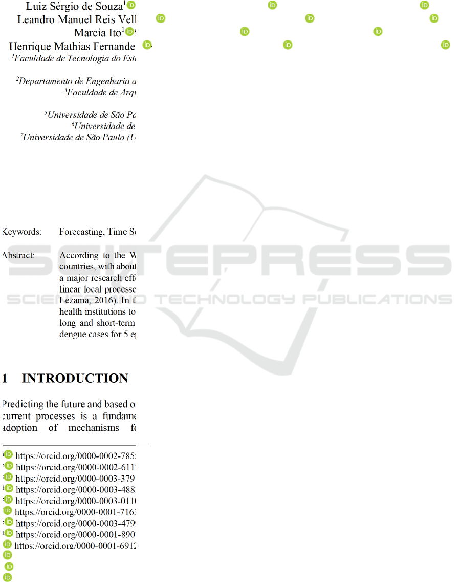
RNNs (Fig. 1) are structures that can scale to very

long-time sequences. The internal states h

of the

processing units of an RNN change as the inputs are

presented over time (t), forming conditions similar to

a memory. RNNs use equation 6 to adjust the values

in their internal processing units. When it is trained to

perform a task that requires predicting the future from

the past, the recurrent network uses h

as a kind of

memory of the relevant aspects of the previous

sequence (x

(t-1)

, x

(t-2)

, x

(t-3)

...) from entries to t.

(Hochreiter and Schmidhuber, 1987).

ℎ



𝑓



ℎ



,𝑥





(6)

DeLTA 2022 - 3rd International Conference on Deep Learning Theory and Applications

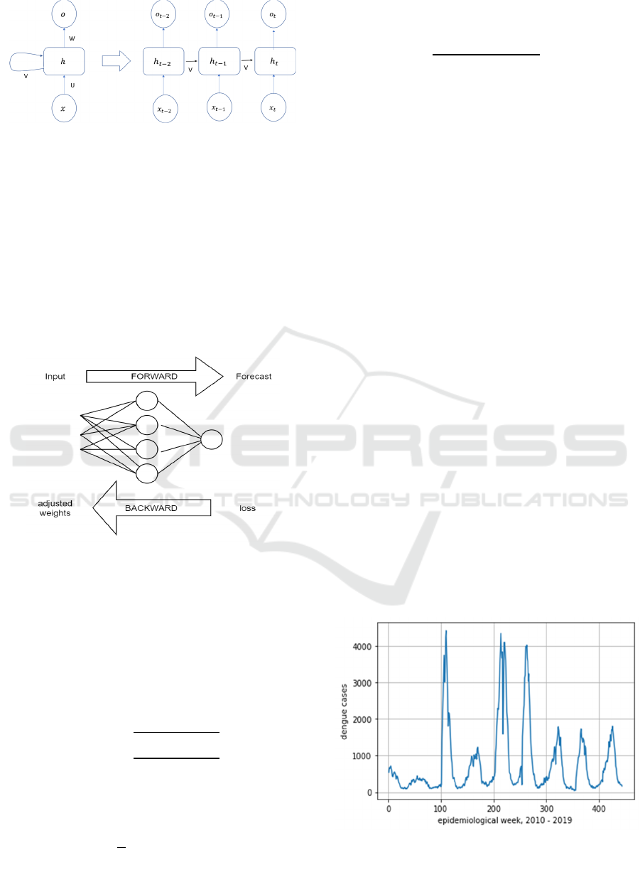
Figure 1: Graph of a Recurring Neural Network.

A. Perceptrons Layers - PL

PL (Fig.2) are structures with feedforward architecture

of processing elements (artificial neurons). Most of

the information needed for processing is extracted in

the layer, which encodes them through synaptic

weights and thresholds of its neurons. The network

training process is usually performed with the

backpropagation algorithm, which uses input and

output pairs to adjust the weights and thresholds of the

network employing an error correction mechanism

(Haykin, 2009).

Figure 2: Graph of a PL.

B. Evaluation Metrics

Building prediction models based on ML demand the

adjustment of parameters such as learning rate,

number of neurons, and sampling window to

minimize the loss function (evaluation metrics)

related to the training process (Faceli et al., 2011).

The most popular loss metrics are:

Root Mean Squared Error – RMSE:

𝑅𝑀𝑆𝐸=



∑

𝑦



−𝑦́











𝑛

(7)

Mean Absolute Error - MAE:

𝑀𝐴𝐸=

𝑛



𝑦



−𝑦́







(8)

Mean Absolute Percentage Error - MAPE:

𝑀𝐴𝑃𝐸=

∑





𝑦



−𝑦





𝑦











𝑛

∙ 100

(9)

Where 𝑦



𝑒 𝑦́



denote the observed value and the

estimated value of the model, respectively, and n is

the number of samples used.

C. Software to Forecast Study

The forecast study was performed using the Keras-

TensorFlow package (Chollet, 2017). The other

packages employed were (i) Pandas libraries for

structuring the data, (ii) Matplotlib for constructing

graphs, (iii) scikit-learn for linear regression and

normalization of the data, and (iv) NumPy for the

vector structure and mathematical functions (Géron,

2017). The version of the software used was the latest

version available on March 15, 2021, in the Python

Package Index (PyPI), for the programming language

Python 3.6. All the software used is free and open

source.

3 FORECAST MODELING

Fig. 3 shows the reported dengue cases by

epidemiological week, counted from 2011 to 2020 for

a Brazilian city with a demographic density of

1.8 hab/km² and was carried out based on information

available in the SINAN (Sistema de Informação de

Agravos de Notificação) (SINAN, 2022). The time

series histogram is shown in Fig. 4. In previous

experiments, a considerable loss for forecast model

accuracy was found for highest incidence values

because of sampling bias for smaller values. Fig. 5

and 6 shows the time series and histogram with the

logarithmic function.

Figure 3: Dengue cases by epidemiological week, counted

from 2010 to 2020 for a Brazilian city with a demographic

density of 1.8 hab/km².

Forecast of Dengue Cases based on the Deep Learning Approach: A Case Study for a Brazilian City

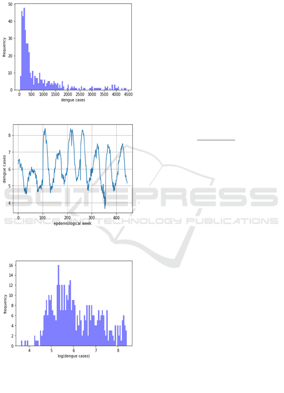
Figure 4: Histogram of the dengue time series.

Figure 5: Dengue cases by epidemiological week, counted

from 2010 to 2020 for a Brazilian city with a demographic

density of 1.8 hab/km² - logarithmic function.

Figure 6: Histogram of the dengue time series - logarithmic

function.

D. Sampling Window

Determining the sampling window to be used as input

for the forecast model is not trivial, especially when

working with data visualization platforms, in which

the user can choose a new time series for the

projection at any time. The algorithm must, therefore,

adapt different models for the forecast horizon in

question, according to the real data of the chosen

series as input to the neural network. For this, we

propose to use lags to the forecast horizon, H, for

which the values of the Autocorrelation Function

(ACF) are greater in module than the statistical

confidence limits (Samohyl, 2009).

The ACF measures the correlation degree of a

variable with itself in previous time units (lag),

allowing to infer the long term of the time series

(Samohyl, 2009). The autocorrelation coefficient for

the lag, θ, is given by:

𝑟



𝐶𝑜𝑣



𝑋



,𝑋





𝑉𝑋





(10)

where 𝐶𝑜𝑣



𝑋



,𝑋





is the covariance of the

series values lagged by 𝜃 and 𝑉



𝑋





the variance at t.

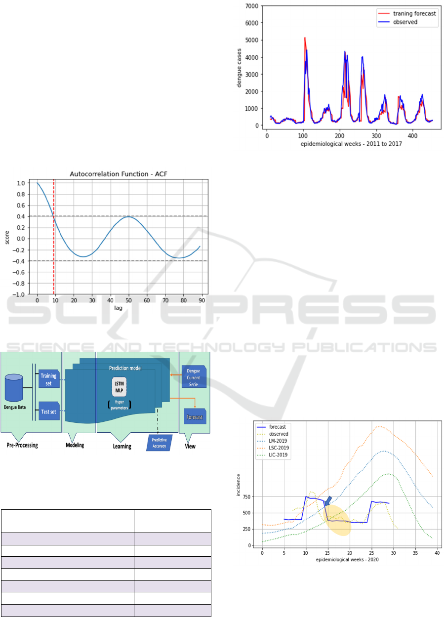
Fig. 7 shows the ACF for the dengue cases series

of the Brazilian city studied. The score for lags greater

than 10 epidemiological weeks tends to values

between 0.4 and -0.4, which, according to Samohyl

(2009), are considered of lesser statistical

significance . Thus, for this series, the lags for the

sampling window are 𝑥



, 𝑥



... 𝑥



The metrics defined in eq. 7, 8, and 9 are generally

used in TSF applications but with different behaviors.

For example, MAE and MAPE are very smooth when

the average error is small. Conversely, the RMSE is

highly sensitive to outliers. A cost function that

combines the best properties of these metrics is the

logcosh function (Chollet, 2017) that works as the

RMSE, but is attenuated for outliers. Thus, the

logcosh cost function was used in all the models

implemented in the research.

As proof of concept, in Fig. 8, the input data consist

of the log-values of the dengue cases. The output data

are the forecasting dengue cases in the subsequent

weeks (forecast horizon - H). This implementation

uses an RNN and was named LSTM – PL Model. It

has an input layer corresponding to the records of

dengue cases in the lag window, a hidden layer

containing 70 LSTM cells, and a second hidden PL

with 64 neurons and a dropout rate of 0.5, used to

minimize the overfitting. Finally, the output layer

provides the dengue cases forecast. Table 1 shows the

LSTM-PL Model average loss for different forecast

horizons (H) in the training step. In this research, we

considered the five-week epidemiological forecast

horizon as a useful value for decision making, still

maintaining an acceptable loss rate.

DeLTA 2022 - 3rd International Conference on Deep Learning Theory and Applications

The learning rate determines the adjustment for the

neural network weights when using the Descending

Gradient Method (DGM) in the training stage. In this

research, the Adam version of the DGM was used

with an adaptive learning rate. According to Haikin

(2009), the method is computationally efficient,

requires less memory, is invariant for the diagonal

scaling of gradients and is suitable for problems with

large amounts of data.

To find the best learning rate, experiments were

started with the value of 0.001 and then other values

were verified. For a five-week epidemiological

forecast horizon, the best learning rate was observed

to be 0.01. Fig. 9 shows the forecast of the LSTM-

PL Model versus observed values, for the training set.

Figure 7: ACF for the dengue cases series of a Brazilian city

studied.

Figure 8: Proof of concept.

Table 1: LSTM-PL Model average loss versus forecast

horizons (H).

ORECAST HORIZON

(

WEEKS

) Average loss (%)

3 4.9

4 5.3

5 6.9

6 10.3

7 20.8

8 43.5

9 50.6

Figure 9: Forecast of the LSTM-PL Model for the training

set.

4 RESULTS

Fig. 10 presents the predicted cases for visualizations

carried out from the 20th to the 40th epidemiological

week of 2020, with a forecast horizon of 5 weeks for

each observation (observations indicated by the

arrow).). The LSTM-PL Model average predictive

accuracy using the MAPE (section II, B) metric is

93%. The control chart has a central curve (MCL)

that, in this research, represents the average behavior

of the incidence of dengue in the previous

epidemiological period (52 weeks). This curve is

close to two others that are determined according to

the variability (standard deviation) of the data in the

time series, called Upper Control Limit (UCL) and

Lower Control Limit (LCL). In this research we use

the Exponentially Weighted Moving Average

(EWMA), discussed in Montgomery (2009), to

calculate the MCL, LCL, and UCL control curves.

Figure 10: Control Diagram for dengue cases and the

forecast given by the LSTM-PL Model for 5

to 40

epidemiological week, 2020.

Forecast of Dengue Cases based on the Deep Learning Approach: A Case Study for a Brazilian City

In Fig. 10, the control chart shows early and

consistently a likely occurrence of case

underreporting, for observations carried out from the

14th week. Thus, the alert, duly validated by other

indicators, would give the manager the opportunity to

trigger corrective actions 5 weeks in advance.

5 CONCLUSIONS

In this research, we implemented a model based on

ML to make predictions of dengue cases and present

them in control charts that we intend to make

available in dashboards of digital health platforms.

The use of ACF proved to be a practical approach

for determining the sampling window (lag). This

method is easy to automate for use on digital health

platforms. Note that we use weekly measurements,

which leads to great data variability over time.

However, we believe that this granularity is the most

suitable for timely decision-making.

It is not uncommon for epidemic outbreaks to

occur suddenly and unexpectedly. However, even

when out of control, epidemic outbreaks do not occur

by chance, and the effort to analyze time series is

justified precisely to anticipate and prevent them.

For predicting non-stationary time series, as is the

case of dengue, it is crucial to capture the long-term

dependence contained in the data. Periodic patterns

can be difficult to recover, but the results from this

research show that this can be achieved by ML-based

models. In contrast to classic statistical

methodologies, such as ARIMA and SARIMA

modeling (Cortes et al, 2018), the proposed solution

requires very little intervention by the analyst.

ACKNOWLEDGEMENTS

This research was funded by Pan American Health

Organization – World Health Organization (PAHO -

WHO). The authors would like to acknowledge the

support of the Department of Monitoring and

Evaluation of SUS of the Executive Secretariat of the

Brazilian Ministry of Health (DEMAS/SE-MS), on

behalf of its coordinating officers, Dr. Márcia Ito, and

Átila Szczecinski Rodrigues

REFERENCES

Adhikari b. et al. (2019). Epideep: Exploiting embeddings

for epidemic forecasting. Proceedings of the ACM

SIGKDD International Conference on Knowledge

Discovery and Data Mining. https://doi.org/10.1145/

3292500.3330917

Anggraeni, W. et al. (2018). Artificial Neural Network for

Health Data Forecasting, Case Study: Number of

Dengue Hemorrhagic Fever Cases in Malang Regency,

Indonesia. Proceedings of 2018 International

Conference on Electrical Engineering and Computer

Science, ICECOS 2018, 17, 2019, 207–212. DOI:

<https://doi.org/10.1109/ICECOS.2018.8605254>.

Chollet, F. (2017). Deep Learning with Python. New York,

NY. Ed. Manning Publications

Cortes, F. et al. (2018). Time series analysis of dengue

surveillance data in two brazilian cities. Acta tropica,

Elsevier, v. 182. 12, 13

De la Sante O. (2021). Forecasting in communicable

diseases. WHO, Regional office for the Eastern

Mediterranean. http:// applications.emro.who.int/docs/

em_RC46_8_en.pdf,1999. Accessed in 03/2021

Faceli, K. et al. (2011). Inteligencia Artificial-Uma

abordagem de Aprendizado de Máquina. Ed. LTC.

Falcón-lezama J. et al. (2016). Day-today population

movement and the management of dengue epidemics.

B Math Biol 2016; 78: 2011-2033.

Géron, A. (2017). Hands-on Machine Learning with Scikit-

Learn, Keras, and TensorFlow, 2nd Edition. O’Reilly

Media.

Haykin, S. (2009). Neural Networks. Ed. Prentice Hall.

Hochreiter, S.; schmidhuber, J. (1997). Long Short-Term

Memory; MIT Press: Cambridge, MA, USA, 1997;

Volume 9, pp. 1735–1780.

Montgomery, D. (2009). Introdução ao controle estatístico

da qualidade. Rio de Janeiro: LTC.

Samohyl, R. W. (2009). Controle Estatístico de Qualidade.

Ed Campus.

Sprent P. and Smeeton N. C. (2016). Applied

nonparametric statistical methods. CRC Press.

SINAN. Ministério da Saúde. Sistema De Informação De

Agreavos De Notificação – SINAN (2020).

https://portalsinan.saude.gov.br/

Wang, Y. et al. (2015) Artificial neural networks for

infectious diarrhea prediction using meteorological

factors in Shanghai (China). Appl Soft Computing,

35:280–290.

Xu, J. et al. (2020). Forecast of Dengue Cases in 20

Chinese Cities Based on the Deep Learning

Method. Int. J. Environ. Res. Public Health 2020, 17,

453. https://doi.org/10.3390/ijerph17020453

DeLTA 2022 - 3rd International Conference on Deep Learning Theory and Applications