On the Helmholtz’s Equation Model for Light Propagation in the Cornea
Ad
´
erito Ara
´
ujo
1 a
, S
´
ılvia Barbeiro
1 b
and Milene Santos
2
1
CMUC, Department of Mathematics, University of Coimbra, Portugal
2
Department of Mathematics, University of Coimbra, Portugal
Keywords:
Helmholtz’s Equation, Light Propagation, Cornea, Discontinuous Galerkin Method, Curved Domains.
Abstract:
To model the incidence and reflection of light in the cornea we can use Maxwell’s equations, which describe
the electromagnetic wave’s propagation field. In this paper we will focus on Maxwell’s equations in the time
harmonic form which translates in the Helmholtz’s equation. We propose a numerical method based on nodal
discontinuous Galerkin methods combined with a strategy which is specially designed to deal with curved
domains which arise naturally in our domain of interest for the application.
1 INTRODUCTION
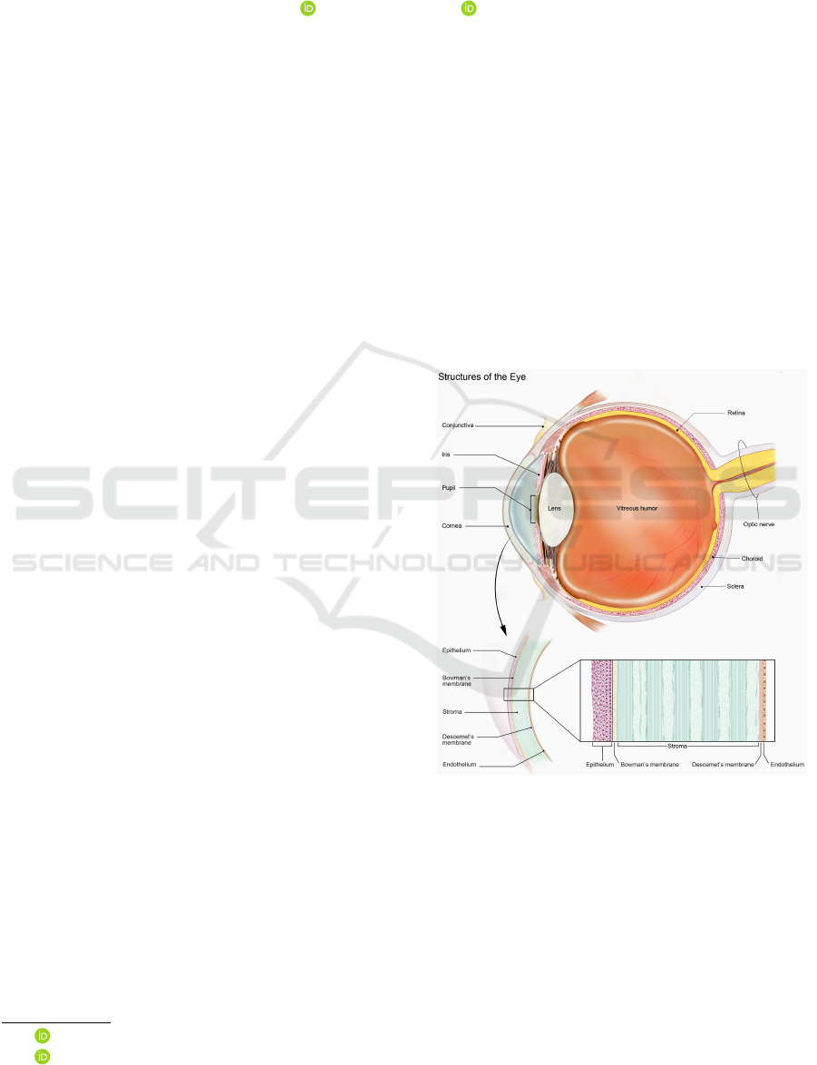
The cornea (see Figure 1) corresponds to the trans-
parent part of the outer layer of the eye and its curved
interface provides three-quarters of the eye’s focusing
power (the rest being provided by the lens). Thus,
maintaining corneal curvature and transparency is es-
sential for good vision, which is translated by less
light reflection and therefore more information is cap-
tured.
The reasons that lead to corneal opacity are not
yet completely determined, but there is consensus that
corneal transparency is related to the shape, size and
organisation of the of the stromal extracellular matrix
and its elements, in particular collagen fibrils and their
refractive indices, which translate the speed of light as
it passes through the medium in question (see (Doutch
et al., 2008), (Farrell et al., 1990), (Meek and Knupp,
2015) and the references therein). Maxwell’s equa-
tions, which describe the electromagnetic field propa-
gation, can be used to model incidence and reflection
of light in the cornea. In this paper we will focus on
Maxwell’s equations in time harmonic form, and con-
sequently, our formulation is based on Helmholtz’s
equation.
We will use a discontinuous Galerkin method
(DG) to solve the Helmholtz equation (Hesthaven and
Warburton, 2008). The DG method admits discontin-
uous solutions and it is a method with a high order
of accuracy scheme. Moreover, being a local method
a
https://orcid.org/0000-0002-9873-5974
b
https://orcid.org/0000-0002-2651-5083
Figure 1: Anatomy of the human eye with corneal cross-
section.
Author: National Eye Institute (licensed under CC BY 2.0).
it allows great flexibility when considering complex
meshes. Analogously to the numerical flow in the
finite volume method, which transports information
from one local element to another, the numerical flow
in the DG method connects adjacent elements, allow-
ing to build the global approximation.
Since we intend to solve the equation in a domain
that mimics the cornea, polygonal meshes do not ex-
actly fit the curved physical domain, thus reducing the
the accuracy of the method. In order to overcome this
Araújo, A., Barbeiro, S. and Santos, M.
On the Helmholtz’s Equation Model for Light Propagation in the Cornea.
DOI: 10.5220/0011126000003209
In Proceedings of the 2nd International Conference on Image Processing and Vision Engineering (IMPROVE 2022), pages 265-268
ISBN: 978-989-758-563-0; ISSN: 2795-4943
Copyright
c
 2022 by SCITEPRESS – Science and Technology Publications, Lda. All rights reserved
265

problem, we will equip our numerical scheme with an
optimisation method based on polynomial reconstruc-
tion (Costa et al., 2018).
This work is part of a more general problem
that consists in understanding the physical basis for
analysing the corneal transparency (Ara
´
ujo et al.,
2022).
2 ELECTROMAGNETIC WAVE
EQUATION
Maxwell’s equations are the fundamental set of equa-
tions that describe how the electromagnetic field
propagates in free space and in any media. Assuming
the electric and magnetic fields to be time harmonic,
E(x,t) = e
iωt
ˆ
E(x) and H(x,t) = e
iωt
ˆ
H(x),
Maxwell’s equations can be written in the form,
iωε
r
ˆ
E = ∇ ×
ˆ
H, iωµ
r
ˆ
H = −∇ ×
ˆ
E, (1)
∇ · ε
r
ˆ
E = 0, ∇ · µ
r
ˆ
H = 0. (2)
Equations (1) and (2) can be reduced to the
Helmholtz’s equation
−∇
2
ˆ
H
z
(x,y) = ω
2
µ
r
ε
r
ˆ
H
z
(x,y), (3)
if we assume an homogeneous media and consider the
TE-mode Maxwell’s equations in 2D.
3 THE DG METHOD
To simplify the notation, let us consider equation (3)
with a source term in the form
−∇
2
u(x) − k
2
u(x) = f (x), x ∈ Ω, (4)
u(x) = 0, x ∈ ∂Ω,
where Ω ⊂ R
2
and x = (x,y). Let Ω
h
be a confor-
mal triangulation of Ω. Introducing a slack variable
q = (q
x
,q
y
)
T
such that q = ∇u, equation (4) can be
written, in each triangle T
k
of Ω
h
, in the form
−∇ · q(x) − k
2
u(x) = f (x), q(x) = ∇u(x).
We thus seek an approximation (u
k
h
,q
k
h
) to (u,q) of
the form
u
k
h
(x) =
N
p
∑
i=1
u
k
h
(x
k
i
)`
k
i
(x)
and
q
k
h,v
(x) =
N
p
∑
i=1
q
k
h,v
(x
k
i
)`
k
i
(x), v = x, y.
where `
k
i
(x) is the Lagrangian polynomial of degree
N defined on T
k
by the grid points x
k
i
, i = 1,...,N
p
,
with N
p
= (N + 1)(N + 2)/2.
Following (Hesthaven and Warburton, 2008), we
conclude that the DG solution can be obtained by
solving a system of linear equations
− ∇S
k
q
k
h
+
Z
∂T
k
ˆ
n ·

q
k
h
− q
∗
h

`
k
dx − k
2
M
k
u
k
h
= M
k
f
h
,
M
k
q
k
h,x
= S
k
x
u
k
h
−
Z
∂T
k
ˆn
x

u
k
h
− u
∗
h

`
k
(x) dx,
M
k
q
k
h,y
= S
k
y
u
k
h
−
Z
∂T
k
ˆn
y

u
k
h
− u
∗
h

`
k
(x) dx,
where ∂T
k
represents the boundary of T
k
, u
k
h
=
[u
k
h
(x
k
i
,y
k
i
)]
N
p
i=1
, q
k
h,v
= [q
k
h,v
(x
k
i
,y
k
i
)]
N
p
i=1
, v = x, y,
`
k
(x) = [`
k
i
(x)]
N
p
i=1
, and, for i, j = 1,...,N
p
,
M
k
i j
=
Z
T
k
`
k
i
(x)`
k
j
(x) dx, ∇S
k
=
h
S
k
x
,S
k
y
i
,
S
k
v,i j
=
Z
T
k
`
k
i
(x)∂`
k
j
(x)/∂v dx, v = x, y.
The numerical fluxes are given by (Hesthaven and
Warburton, 2008)
q
∗
h
= {{∇u
k
h
}}, u
∗
h
= {{u
k
h
}},
where the average
{{u}} =
u
−
+ u
+
2
.
We refer to the interior information of the element by
a superscript “ − ” and to the exterior information by
a superscript “ + ”.
It is well know that the accuracy of the numer-
ical method may be dramatically reduced when the
boundary of the domain Ω is curved. In the next sec-
tion we will consider an adaptation to the numerical
scheme in order to preserve the optimal order of the
DG method.
4 NUMERICAL SETTING
Since we are interested in simulating diverse scenar-
ios which correspond to different kinds of organisa-
tion of the fibrils, polygonal domains don’t fit on our
regions of interest. In particular, we want to consider
healthy and pathological scenarios that correspond to
the organisation of the fibres represented in Figure 2.
A way to deal with curved boundaries is to con-
sider the so-called isoparametric elements, introduced
by Bassi and Rebay in the context of DG methods
(Bassi and Rebay, 1997). The elements are called
isoparametric, since the same functions are used to
Imaging4OND 2022 - Special Session on New Developments in Imaging for Ocular and Neurodegenerative Disorders
266

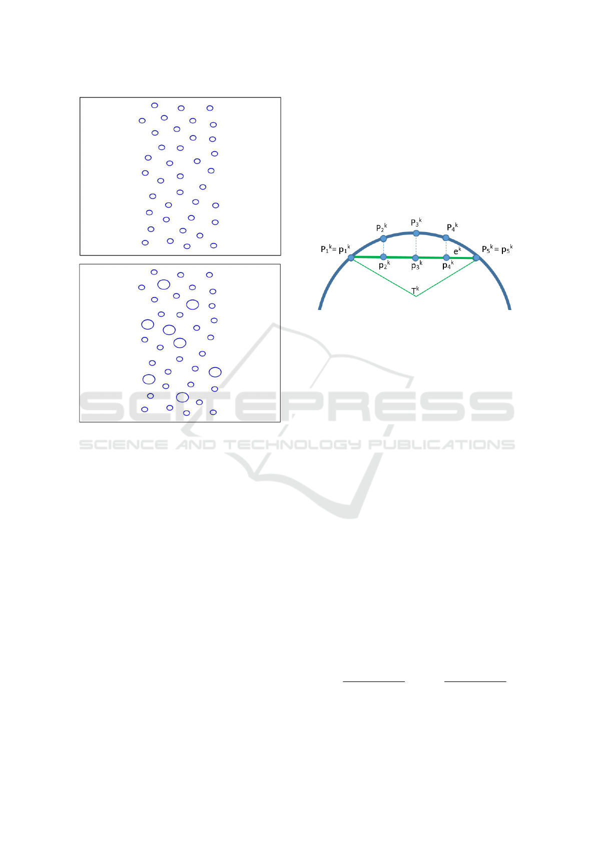
Figure 2: Stromal collagen fibres arrangement (Ara
´
ujo
et al., 2022). Top: healthy cornea; Bottom: cornea with
some fibres whose diameter is doubled.
express the transformation from the reference element
to the real element and the solution in the reference el-
ement. This approach requires the use of non-linear
transformations of the reference triangle, which re-
quires high computational effort. In addition, it re-
quires the generation of curved meshes, which turns
out to be impractical for complex geometries. In or-
der to avoid nonlinear transformations, alternative ap-
proaches have been proposed, namely in the context
of the finite volume method (see (Costa et al., 2018)
and the references therein). In that work, a method
called ROD (Reconstruction for Off-site Data) was
considered. As the name of the method suggests, a
polynomial reconstruction is developed which takes
into account the real boundary conditions (which are
not in the polygonal computational domain). This
method does not require the generation of curved
meshes to adjust the boundary, nor complex nonlinear
transformations, which contributes for computational
efficiency and simplifies the numerical schemes.
We now intend to generalize this approach to the
DG method. The DG-ROD method starts with an iter-
ation of the DG method, obtaining, for each T
k
∈ T
h
,
the polynomial u
k
h
. After this first iteration, for each
T
k
element with an edge e
k
that intersects the bound-
ary (see Figure 3), we determine a polynomial π
k
that
satisfies the boundary condition at a set of points on
the boundary (Costa et al., 2018). Then we update
the DG solution by imposing that on this edge e
k
the
boundary condition is given by the value of π
k
. The
procedure is repeated for a certain number of itera-
tions.
Figure 3: Example of an element T
k
with an edge that in-
tersects the boundary and a set of 5 points on the boundary.
The results obtained by the DG-ROD method are
very encouraging and prove its effectiveness. We start
by considering a particular example of (4) with k = 1,
defined on a circular domain, with known exact so-
lution u and apply both DG and DG-ROD. In partic-
ular, we are considering a simplified problem where
the medium can be described by a circle of radius 1
centred at the origin and no internal fibrils.
If we denote by u
h
an approximate solution de-
termined with the numerical method, we say that the
method has order of convergence p if
||u − u
h
|| ≤ Ch
p
,
for a given norm k · k, with C a real constant indepen-
dent of h.
In order to estimate the order of convergence of
both methods, we considered different spatial meshes
generated by Gmsh (Geuzaine and Remacle, 2020),
with different mesh parameters h. Considering two
distinct values of h, say h
1
and h
2
, we compute the
maximum norms
E
∞,1
= ||u − u
h
1
||
∞
and E
∞,2
= ||u − u
h
2
||
∞
.
Assuming
E
∞,1
/E
∞,2
= (h
1
/h
2
)
p
,
we have that the order of convergence can be esti-
mated by
p =
log(E
∞,1
/E
∞,2
)
log(h
1
/h
2
)
⇒ p ≈ 2
log(E
∞,1
/E
∞,2
)
log(K
2
/K
1
)
with K
i
the number of triangles of the mesh i, for i =
1,2, where h
1
/h
2
≈ (K
2
/K
1
)
1/2
.
On the Helmholtz’s Equation Model for Light Propagation in the Cornea
267

The results obtained in our simulations by the
DG method and by the iterative DG-ROD method for
polynomials of degree N, with N = 1,2,3,4, show
that the order of convergence for the DG method is
p = 2 and for the DG-ROD method the order is p = N.
We then proved that the DG-ROD method, unlike the
classical DG method, allows to obtain high order in
domains with curved boundary.
5 CONCLUSIONS
In this paper we discuss an approach for dealing with
the decreased accuracy of discontinuous Galerkin fi-
nite element method (DG) in domains with curved
boundary. Following (Costa et al., 2018), we consider
an approach based on the polynomial reconstruction
of the boundary condition imposed on the computa-
tional domain, where the associated parameters are
determined such that the reconstructions adequately
satisfies the boundary condition imposed in the real
domain. The overall method consists on an iterative
method that considers two independent steps: solving
the differential equation by the classical DG and the
reconstruction process on the triangles with vertex on
the boundary of the real curved domain. The numeri-
cal results obtained show the efficiency of the method,
i.e., it is able to achieve high order of precision in do-
mains with curved boundaries.
ACKNOWLEDGEMENTS
The design, analysis, interpretation of data and
writing of the manuscript have been supported
by the Centre for Mathematics of the Univer-
sity of Coimbra - UIDB/00324/2020, funded by
the Portuguese Government through FCT/MCTES,
and by FCT/MCTES through the project refer-
ence PTDC/MAT-APL/28118/2017 and POCI-01-
0145-FEDER-028118.
REFERENCES
Ara
´
ujo, A., Barbeiro, S., Bernardes, R., Morgado, M.,
and Sakic, S. (2022). A mathematical model for the
corneal transparency problem. Accepted for publica-
tion in Journal of Mathematics in Industry.
Bassi, F. and Rebay, S. (1997). High-order accurate discon-
tinuous finite element solution of the 2d euler equa-
tions. Journal of Computational Physics, 138:251–
285.
Costa, R., Clainb, S., Loubr
`
ec, R., and J. Machado,
G. (2018). Very high-order accurate finite vol-
ume scheme on curved boundaries for the two-
dimensional steady-state convection–diffusion equa-
tion with Dirichlet condition. Applied Mathematical
Modelling, 54:752–767.
Doutch, J., Quantock, A. J., Smith, V. A., and Meek, K. M.
(2008). Light transmission in the human cornea as a
function of position across the ocular surface: Theo-
retical and experimental aspects. Biophysical Journal,
95:5092–5099.
Farrell, R. A., Freund, D. E., and Mccaly, R. L. (1990).
Research on corneal structure. Johns Hopkins APL
Technical Digest, 11(1-2):191–199.
Geuzaine, C. and Remacle, J.-F. (2020). Gmsh.
http://http://gmsh.info/. version 4.6.0.
Hesthaven, J. and Warburton, T. (2008). Nodal Discontin-
uous Galerkin Methods: Algorithms, Analysis, an Ap-
plications. Springer-Verlag, New York.
Meek, K. M. and Knupp, C. (2015). Corneal structure and
transparency. Progres in Retinal and Eye Research,
49:1–16.
Imaging4OND 2022 - Special Session on New Developments in Imaging for Ocular and Neurodegenerative Disorders
268