On the Numerical Solution of the Inverse Elastography Problem for
Time-harmonic Excitation
Pedro Serranho
1,2 a
, S
´
ılvia Barbeiro
3 b
, Rafael Henriques
3 c
, Ana Batista
2 d
, M
´
ario J. Santos
4 e
,
Carlos Correia
2 f
, Jos
´
e P. Domingues
5 g
, Cust
´
odio Loureiro
5 h
, Jo
˜
ao M. R. Cardoso
5 i
,
Rui Bernardes
2,6 j
and Miguel Morgado
2,5 k
1
Department of Science and Technology, Universidade Aberta, Rua da Escola Polit
´
ecnica, 147, 1269-001, Lisbon, Portugal
2
Coimbra Institute for Biomedical Image and Translational Research, Faculty of Medicine, University of Coimbra,
Edif
´
ıcio do ICNAS, Polo 3 Azinhaga de Santa Comba 3000-548, Coimbra, Portugal
3
University of Coimbra, CMUC - Center of Mathematics, Department of Mathematics, Apartado 3008,
EC Santa Cruz, 3001-501, Coimbra, Portugal
4
University of Coimbra, Department of Electrical and Computer Engineering, Faculty of Science and Technology,
P
´
olo II, 3030-290, Coimbra, Portugal
5
Department of Physics, University of Coimbra, Rua Larga, 3004-516, Coimbra, Portugal
6
University of Coimbra, CACC-Clinical Academic Center of Coimbra, Faculty of Medicine (FMUC), Coimbra, Portugal
Keywords:
Numerical Methods, Method of Fundamental Solutions, Elastography, Optical Coherence Elastography.
Abstract:
In this paper we address the numerical solution of the inverse elastography problem, from the knowledge of
the excitation field on the boundary and the displacement field in a grid of points within the domain. We
suggest using a representation of the solution by the method of fundamental solutions and using a Newton-
type method to iteratively approximate the Lam
´
e coefficients of the medium from elastography displacement
measurements. We consider a toy model to illustrate the performance of the method.
1 INTRODUCTION
Elastography is an imaging modality where the elas-
tic displacement induced by a given excitation on the
imaged tissue is measured to recover the material’s
elastic properties.
We are especially interested in considering optical
coherence elastography (OCE), which means that one
used optical coherence tomography to measure the
a
https://orcid.org/0000-0003-2176-3923
b
https://orcid.org/0000-0002-2651-5083
c
https://orcid.org/0000-0003-4173-8469
d
https://orcid.org/0000-0002-5672-8266
e
https://orcid.org/0000-0002-0188-7761
f
https://orcid.org/0000-0002-2947-1880
g
https://orcid.org/0000-0002-0562-8994
h
https://orcid.org/0000-0001-7856-2124
i
https://orcid.org/0000-0002-8832-8208
j
https://orcid.org/0000-0002-6677-2754
k
https://orcid.org/0000-0001-9455-1206
phase difference related to the elastic movement and
the consequent elastic displacement in depth of the
tissue (see, for instance (Claus et al., 2017; Kennedy
et al., 2011; Qu et al., 2018; Zhu et al., 2017)). There-
fore, one is interested in recovering the elastic prop-
erties of the tissue material given the measurement of
the depth displacement in a grid of inner points within
the tissue and the time-harmonic excitation.
This paper will consider time-harmonic excitation
for the Lam
´
e equation, which allows the elastic field
to be represented by the method of fundamental so-
lutions (MFS). In this case, we propose a Newton’s
method approach based on the differentiation of the
operator that maps the Lam
´
e coefficients to the solu-
tion of the problem. At each iteration the proposed
method requires few computational effort to update
the Lam
´
e coefficients, since it resumes to solve a 2-
by-2 linear system at each iteration. However, to es-
tablish this linear system a forward problem must be
solved at each iteration, which supports the choice of
a MFS approach due to its easy implementation. We
Serranho, P., Barbeiro, S., Henriques, R., Batista, A., Santos, M., Correia, C., Domingues, J., Loureiro, C., Cardoso, J., Bernardes, R. and Morgado, M.
On the Numerical Solution of the Inverse Elastography Problem for Time-harmonic Excitation.
DOI: 10.5220/0011125900003209
In Proceedings of the 2nd International Conference on Image Processing and Vision Engineering (IMPROVE 2022), pages 259-264
ISBN: 978-989-758-563-0; ISSN: 2795-4943
Copyright
c
 2022 by SCITEPRESS – Science and Technology Publications, Lda. All rights reserved
259

also discuss the main advantages and possible disad-
vantages of this approach.
2 PROBLEM FORMULATION
For time-harmonic waves, the Lam
´
e equation governs
the elastic displacement field u in a domain D (Doy-
ley, 2012; Park and Maniatty, 2006) by
µ∆u + (λ+ µ) grad divu + ω
2
ρu = 0 in D, (1)
where ρ is the density, ω is the frequency, and the
Lam
´
e constants are given by
µ =
E
2(1 + υ)
, λ =
υE
(1 + υ)(1 − 2υ)
,
where υ is the Poisson’s ratio and E is the Young’s
Modulus. Usually in this setting the boundary condi-
tions are defined by the pressure p, namely by relating
it with the elastic field u at some part Γ of the bound-
ary δD by one or both of the following transmission
conditions (Ito et al., 2008; Ito and Toivanen, 2007)
1
ρ
∂ p
n−1
∂ν
= ω
2
u · ν on Γ, (2)
p
n−1
ν
n−1
= σ(u)ν
n
on Γ, (3)
where the stress tensor is given by
σ(u) = µ(∇u + (∇u)
T
) + λdivuI.
In the remaining boundary, one can assume either
u = 0 on ∂D \ Γ (4)
or
σ(u)ν = 0 on ∂D \ Γ. (5)
The setting of the problem is illustrated in figure 1.
Figure 1: Problem and Domain setting.
The direct problem consists in determining the
elastic field u within the domain D, given the pres-
sure p on Γ, the material’s density ρ, the frequency ω
and Lam
´
e coefficients µ and λ. This can be done us-
ing a forward solver as for instance the MFS, which
we will detail in the following section.
The inverse problem consists in determining the
Lam
´
e coefficients µ and λ from the knowledge of elas-
tic field u in a discrete grid of points in domain D, the
pressure p on Γ, the material’s density ρ and the fre-
quency ω. The following section will address the pro-
posed numerical approach based on Newton’s method
to solve the inverse problem.
3 NUMERICAL METHOD
Having in mind that the fundamental solution of equa-
tion (1) in R
2
is given by (cf. (Alves et al., 2017))
Φ(x) =
i
4ρω
2

κ
2
s
H
(1)
0
(κ
s
|x|)I
+grad grad(H
(1)
0
(κ
s
|x|) − H
(1)
0
(κ
p
|x|))

(6)
where
κ
2
p
=
ω
2
ρ
λ + 2µ
, κ
2
s
=
ω
2
ρ
µ
, (7)
H
(1)
n
is the Hankel function of first kind and order n, I
is the identity operator in R
2
and one has
gradgrad(H
(1)
0
(κ|x|) =κ
2
x.x
T
|x|
2
H
(1)
2
(κ|x|)
−
κ
|x|
H
(1)
1
(κ|x|)I,
the method of fundamental solutions is based on the
representation of the solution as
u(x;κ
s
,κ
p
) =
N
s
∑
k=1
Φ

x − s
k

α
k
(8)
for some source points s
k
/∈
¯
D, k = 1, 2,... ,N
s
, and
coefficients α
k
∈ C
2
. From the definition of funda-
mental solution, it can be shown that this representa-
tion fulfils equation (1). Moreover, it can be shown
that solutions of this form are dense for analytic solu-
tions of the problem (Alves et al., 2017).
Therefore, the method of fundamental solutions is
a good choice for forward solver (cf. (Barbeiro and
Serranho, 2020)), since one needs only to find the
coefficients α
k
∈ C
2
such that the boundary condi-
tions (2)-(3) and (4) or (5) are satisfied.
Given the elastography data, that is, the measure-
ment points x
j
∈ D, j = 1, 2, ... , N
m
and the respective
displacement measures u
j
= u(x
j
), we now define the
operators
G
j
: (κ
s
,κ
p
) 7→ u(x
j
;κ
s
,κ
p
) − u
j
, j = 1,2, ... N
m
.
In this way, one wants to find κ
s
,κ
p
such that
G
j
(κ
s
,κ
p
) = 0,∀ j = 1,2, ...N
m
.
Imaging4OND 2022 - Special Session on New Developments in Imaging for Ocular and Neurodegenerative Disorders
260

To achieve this, we propose a Newton’s method ap-
proach. At iteration n, given the current approxima-
tions

κ
(n)
s
,κ
(n)
p

one solves the system of N
m
equa-
tions
∂G
j
∂κ
s

κ
(n)
s
,κ
(n)
p

h
s
+
∂G
j
∂κ
p

κ
(n)
s
,κ
(n)
p

h
p
= −G
j
(κ
(n)
s
,κ
(n)
p
)
with respect to (h
s
,h
p
) in a least square sense, having
the new update
κ
(n+1)
s
= κ
(n)
s
+ h
s
, κ
(n+1)
p
= κ
(n)
p
+ h
p
.
The method is now iterated until some stopping crite-
ria is achieved. It is also worth noting that in this case
one has
∂G
j
∂κ
s
(κ
s
,κ
p
) =
∂u
∂κ
s
(x
j
;κ
s
,κ
p
) (9)
∂G
j
∂κ
p
(κ
s
,κ
p
) =
∂u
∂κ
p
(x
j
;κ
s
,κ
p
) (10)
However, in particular for OCE one only gathers the
displacement in depth, so in this case the operator G
j
should be modified to
G
2, j
: (κ
s
,κ
p
) 7→ u
2
(x
j
;κ
s
,κ
p
) − u
2, j
that is, one has only access to the second component
of the displacement vector.
We also note that the problem of recover-
ing (κ
s
,κ
p
) is equivalent to recovering (µ,λ), since
one pair uniquely defines the other by (7).
4 PRELIMINARY NUMERICAL
RESULTS
The numerical results we present here are ongoing
work, so you will only consider a simple toy model.
Moreover, tunning of the parameters has not yet been
consider, so the results might improve.
We consider D to be a unit circle. Instead of
the boundary conditions (2)-(5), we considered the
Dirichlet boundary condition in all of x ∈ ∂D given
by
u(x) = 0.25 exp(iκd · x)exp(−|x − (0,1)|
2
/0.25)ν
(11)
with d = (−1,−5)/
p
(26), κ = 1 and ν is the out-
ward normal unit vector to the boundary. Also, we
considered ω = ρ = 1. For the forward problem, we
considered 800 collocation equally spaced points over
the unit circumference and 400 source equally spaced
points over the circumference of radius r=1.2, for the
MFS representation (8). We considered Tikhonov
regularization to solve the overdetermined linear sys-
tem to determine α
k
in (8) by imposing (11) on the
collocation points. This procedure obtained the dis-
placement field u
j
in a grid of points x
j
as illustrated
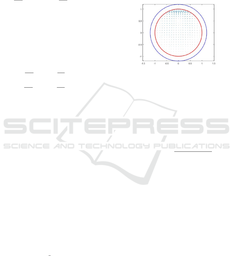
in figure 2, for example 1.
Figure 2: Displacement field data u
j
in the measurement
points x
j
and displacement given by boundary condition for
example 1 (κ
s
= 0.5,κ
p
= 2), with 400 source points (blue)
and 800 collocation points (red).
To avoid an inverse crime (Colton and Kress,
2013), for the inverse problem we considered 200 col-
location points equally spaced over the unit circum-
ference and 100 source points equally spaced over the
circumference of radius r=1.1, for the forward MFS
solver considering the current approximation for the
parameters (κ
(n)
s
,κ
(n)
p
), with the same regularization
parameter.
We considered the error norm
||G
(n)
2
||
`
2
=
v
u
u
t
N
m
∑
j=1
G
2, j
(κ
(n)
s
,κ
(n)
p
)
and stop the algorithm whenever this error increases
from one iteration to the following.We also define the
error in the approximation
e
(n)
s
= |κ
(n)
s
− κ
s
|, e
(n)
p
= |κ
(n)
p
− κ
p
|.
We started by considering κ
s
= 0.5 and κ
p
= 2 in
example 1. The results are shown in Table 1 for exact
data and in Table 2 for multiplicative 1% noise in the
data. We can see that for exact data the approximation
has high precision and is not very affected with noise.
As for example 2, we considered κ
s
= 1.2 and κ
p
= .5,
with results in Table 3 for exact data and in Table 4
for multiplicative 1% noise in the data. In this case
the method seems to stop very early for exact data.
This is clear once for noisy data, the method performs
at a very similar level. Future work should consider
optimization of the regularization coefficient based on
error and/or number of points.
On the Numerical Solution of the Inverse Elastography Problem for Time-harmonic Excitation
261

Table 1: Results for exact data for example 1:κ
s
= 0.5, κ
p
= 2.
n κ
(n)
s
κ
(n)
p
e
(n)
s
e
(n)
p
||G
(n)
2
||
`
2
0 1 1 0.5 -1 0.036015
1 0.85337 1.2119 0.35337 -0.78813 0.022349
5 0.46939 1.4692 -0.030611 -0.53076 0.0041958
10 0.44448 1.588 -0.055522 -0.41196 0.0028442
50 0.49623 1.9429 -0.0037699 -0.057122 0.00047919
100 0.49975 1.9951 -0.00025248 -0.0049319 4.2702e
−5
200 0.50000 2.0000 -1.3591e
−6
-3.3625e
−5
3.1419e
−7
249 0.50000 2.0000 3.3361e
−7
3.5057e
−7
1.0881e
−7
250 0.50000 2.0000 3.4172e
−7
5.1348e
−7
1.0882e
−7
Table 2: Results for 1% noisy data for example 1:κ
s
= 0.5, κ
p
= 2.
n κ
(n)
s
κ
(n)
p
e
(n)
s
e
(n)
p
||G
(n)
2
||
`
2
0 1 1 0.5 -1 0.036014
1 0.85332 1.2117 0.35332 -0.7883 0.022352
5 0.46871 1.4684 -0.031286 -0.53156 0.0041952
10 0.44344 1.5865 -0.056559 -0.4135 0.0028518
50 0.49489 1.9389 -0.0051093 -0.061051 0.00053961
100 0.49845 1.9908 -0.0015487 -0.0092421 0.00020766
200 0.49871 1.9956 -0.0012923 -0.0043913 0.00019709
424 0.49871 1.9956 -0.0012904 -0.0043545 0.00019704
Table 3: Results for exact data for example 2:κ
s
= 1.2, κ
p
= 0.5.
n κ
(n)
s
κ
(n)
p
e
(n)
s
e
(n)
p
||G
(n)
2
||
`
2
0 0.8 0.8 -0.4 0.3 0.02538
1 0.95237 0.70177 -0.24763 0.20177 0.01406
5 1.0882 0.60583 -0.11183 0.10583 0.0057529
10 1.14 0.55603 -0.059973 0.056034 0.0028045
20 1.1719 0.50782 -0.028133 0.0078185 0.00070746
30 1.1779 0.48971 -0.022086 -0.010286 0.00011391
34 1.178 0.48604 -0.021955 -0.013962 8.4068e
−5
Table 4: Results for 1% noisy data for example 2:κ
s
= 1.2, κ
p
= 0.5.
n κ
(n)
s
κ
(n)
p
e
(n)
s
e
(n)
p
||G
(n)
2
||
`
2
0 0.8 0.8 -0.4 0.3 0.025379
1 0.95227 0.70148 -0.24773 0.20148 0.014052
5 1.0877 0.60483 -0.11231 0.10483 0.0057361
10 1.1391 0.55427 -0.060947 0.054272 0.0027864
20 1.1697 0.50482 -0.030252 0.0048246 0.00074093
30 1.1745 0.48572 -0.0255 -0.014282 0.00035822
32 1.1744 0.48353 -0.025616 -0.016473 0.00035996
5 FINAL REMARKS AND
PERSPECTIVES
The application of Newton’s method for inverse prob-
lems is common (Kress, 2003) and convergence as
been proven for some settings of ill-posed inverse
problems (Hohage, 1998; Potthast, 2001). Also, the
idea of using a reconstruction of field using the cur-
rent approximation of the unknowns and a subsequent
iteration based on the derivative of the operator that
Imaging4OND 2022 - Special Session on New Developments in Imaging for Ocular and Neurodegenerative Disorders
262

maps the unknowns to the field has been successfully
used in shape reconstruction of unknown obstacles in
acoustics (Kress and Serranho, 2005; Kress and Ser-
ranho, 2007; Serranho, 2006; Serranho, 2007), so the
use of a similar idea in elastodynamics seems promis-
ing.
The use of MFS for the direct elastography prob-
lem was also successful (Barbeiro and Serranho,
2020), supporting our choice for the ansatz of the
elastic field. However, the solution of the inverse
problem is, as usual, more complex. Newton’s
method worked well on our toy model, but more ex-
periments need to be made. The method seems very
sensitive to the choice of the initial guess (κ
(0)
s
,κ
(0)
p
)
as usually in the application of Newton’s method for
ill-posed problems. In addition, the radius of the cir-
cumference for the source points, the choice of reg-
ularization parameters and the number of colloca-
tion and source points also affect the results. More-
over, we only considered low frequencies. High fre-
quencies increase the ill-posedness and require more
source points, turning the numerical solution more
complex. These aspects should be addressed in future
research.
Finally, domains with corners as in figure 1 or
non-smooth initial conditions will require the enrich-
ment of the basis functions of fundamental solutions
with particular solutions that can cope with those sin-
gularities and discontinuities, in the spirit of (Alves
et al., 2018). This will also be addressed in further
research, since it allows the method to be applied in
a setting as in figure 1 that is closer to elastography
applications.
ACKNOWLEDGEMENTS
The authors would like to acknowledge their work
is partially supported by FEDER Funds through
the Operational Program for Competitiveness Fac-
tors - COMPETE and by Portuguese National Funds
through FCT - Foundation for Science and Tech-
nology under the PTDC/EMD-EMD/32162/2017
project.
REFERENCES
Alves, C. J., Martins, N. F., and Valtchev, S. S. (2017). Ex-
tending the method of fundamental solutions to non-
homogeneous elastic wave problems. Applied Numer-
ical Mathematics, 115:299 – 313.
Alves, C. J., Martins, N. F., and Valtchev, S. S. (2018). Tr-
efftz methods with cracklets and their relation to bem
and mfs. Engineering Analysis with Boundary Ele-
ments, 95:93–104.
Barbeiro, S. and Serranho, P. (2020). The Method of Funda-
mental Solutions for the Direct Elastography Problem
in the Human Retina, pages 87–101. Springer Inter-
national Publishing, Cham.
Claus, D., Mlikota, M., Geibel, J., Reichenbach, T., Pedrini,
G., Mischinger, J., Schmauder, S., and Osten, W.
(2017). Large-field-of-view optical elastography us-
ing digital image correlation for biological soft tissue
investigation. Journal of Medical Imaging, 4(1):1 –
14.
Colton, D. and Kress, R. (2013). Inverse Acoustic and Elec-
tromagnetic Scattering Theory. Springer, 3
rd
edition
edition.
Doyley, M. M. (2012). Model-based elastography: a sur-
vey of approaches to the inverse elasticity problem.
Physics in Medicine and Biology, 57(3):R35–R73.
Hohage, T. (1998). Convergence rates of a regularized new-
ton method in sound-hard inverse scattering. SIAM J.
Numer. Anal., 36:125–142.
Ito, K., Qiao, Z., and Toivanen, J. (2008). A domain
decomposition solver for acoustic scattering by elas-
tic objects in layered media. J. Comput. Phys.,
227(19):8685–8698.
Ito, K. and Toivanen, J. (2007). A fast iterative solver for
scattering by elastic objects in layered media. Ap-
plied Numerical Mathematics, 57(5):811 – 820. Spe-
cial Issue for the International Conference on Scien-
tific Computing.
Kennedy, B. F., Liang, X., Adie, S. G., Gerstmann, D. K.,
Quirk, B. C., Boppart, S. A., and Sampson, D. D.
(2011). In vivo three-dimensional optical coherence
elastography. Opt. Express, 19(7):6623–6634.
Kress, R. (2003). Newton’s method for inverse obstacle
scattering meets the method of least squares. Inverse
Problems, 19:91–104.
Kress, R. and Serranho, P. (2005). A hybrid method for two-
dimensional crack reconstruction. Inverse Problems,
21:773–784.
Kress, R. and Serranho, P. (2007). A hybrid method for
sound-hard obstacle reconstruction. Journal of Com-
putational and Applied Mathematics, 204:418–427.
Park, E. and Maniatty, A. M. (2006). Shear modulus re-
construction in dynamic elastography: time harmonic
case. Physics in Medicine and Biology, 51(15):3697–
3721.
Potthast, R. (2001). On the convergence of a new newton-
type method in inverse scattering. Inverse Problems,
17:1419–1434.
Qu, Y., He, Y., Zhang, Y., Ma, T., Zhu, J., Miao, Y., Dai, C.,
Humayun, M., Zhou, Q., and Chen, Z. (2018). Quan-
tified elasticity mapping of retinal layers using syn-
chronized acoustic radiation force optical coherence
elastography. Biomed. Opt. Express, 9(9):4054–4063.
Serranho, P. (2006). A hybrid method for inverse scattering
for shape and impedance. Inverse Problems, 22:663–
680.
On the Numerical Solution of the Inverse Elastography Problem for Time-harmonic Excitation
263

Serranho, P. (2007). A hybrid method for inverse scattering
for sound-soft obstacles in 3D. Inverse Problems and
Imaging, 4:691–712.
Zhu, J., Miao, Y., Qi, L., Qu, Y., He, Y., Yang, Q., and Chen,
Z. (2017). Longitudinal shear wave imaging for elas-
ticity mapping using optical coherence elastography.
Applied Physics Letters, 110(20):201101.
Imaging4OND 2022 - Special Session on New Developments in Imaging for Ocular and Neurodegenerative Disorders
264