Assess Performance Prediction Systems: Beyond Precision Indicators
Amal Ben Soussia, Chahrazed Labba, Azim Roussanaly and Anne Boyer
Universit
´
e de Lorraine, LORIA, France
Keywords:
Earliness, Stability, Indicators, Learning Analytics, Machine Learning, k-12 Learners.
Abstract:
The high failure rate is a major concern in distance online education. In recent years, Performance Prediction
Systems (PPS) based on different analytical methods have been proposed to predict at-risk of failure learners.
One of the main studied characteristics of these systems is its ability to provide accurate early predictions.
However, these systems are usually assessed using a set of evaluation measures (e.g. accuracy, precision) that
do not reflect the precocity, continuity and evolution of the predictions over time. In this paper, we propose
to enrich the existing indicators with time-dependent ones including earliness and stability. Further, we use
the Harmonic Mean to illustrate the trade-off between the predictions earliness and the accuracy. In order to
validate the relevance of our indicators, we used them to compare four different PPS for predicting at-risk
of failure learners. These systems are applied on real data of K-12 learners enrolled in an online physics-
chemistry module.
1 INTRODUCTION
The use of distance online education has evolved over
the last few years, and has exploded further with the
recent covid-19 pandemic. It presents an effective
way to maintain the continuity of the learning pro-
cess by allowing access to school from anywhere at
any time.
However, the major concern of this learning mode
is the high failure rate among its learners. In order
to meet this issue, Performance Prediction Systems
(PPS) based on Machine Learning (ML) models have
been proposed (Wang et al., 2017; Iqbal et al., 2017;
Zhang et al., 2017; Chui et al., 2020). The main ob-
jective of this type of systems is to predict accurately
and at the earliest at-risk of failure learners using real-
time flow data.
The data generated by online education platforms
are available progressively over time, as they are
highly dependent on the time at which learners inter-
act with the educational content. Thus, these data are
called time series, as they consist of a set of sequences
of events that occur over time. The time reference can
be a timestamp or any other finite-grain time interval
(e.g week). To assess the effectiveness of the PPS in
fulfilling their objectives, common indicators are be-
ing used. On the one hand, performance measures are
used to assess the temporal and space complexity of
the systems in respect to the used data. On the other
hand, ML indicators such as precision, recall and F1
measure are used to qualify the ability of the system
to predict correctly. Despite the diversity of existing
evaluation indicators, none of them is dedicated to as-
sess the precocity, continuity and evolution of predic-
tions over time. However, time is an important di-
mension that needs to be considered while assessing
a PPS as both learning and prediction evolve.
In this paper, we focus on assessing PPS based on
time-series classifiers. To overcome the limitations
of existing common indicators, we focus on provid-
ing new time-dependent ones that can be used to as-
sess these systems over time. Two indicators includ-
ing earliness and stability are proposed. Indeed, the
temporal stability is the ability of a PPS to provide
the longest sequences of correct predictions over the
prediction times. Whereas, the earliness indicates the
first time that the PPS correctly predicted a given class
label. A PPS is said to be effective if it predicts accu-
rately and as early as possible. To this end, we used
the Harmonic Mean (HM) to study the trade-off be-
tween the accuracy and earliness indicators since they
are proportionally inverted.
To validate the relevance of these indicators, we
applied them to assess four different PPS for pre-
dicting at-risk of failure learners. These systems
use real data of k-12 learners enrolled in a physics-
chemistry module within a French distance learning
Ben Soussia, A., Labba, C., Roussanaly, A. and Boyer, A.
Assess Performance Prediction Systems: Beyond Precision Indicators.
DOI: 10.5220/0011124300003182
In Proceedings of the 14th International Conference on Computer Supported Education (CSEDU 2022) - Volume 1, pages 489-496
ISBN: 978-989-758-562-3; ISSN: 2184-5026
Copyright
c
 2022 by SCITEPRESS – Science and Technology Publications, Lda. All rights reserved
489

center (CNED
1
).
To summarize, our contribution is twofold: 1) new
indicators including earliness and stability
; and 2) a real case study to support the use of our
indicators.
The rest of the paper is organized as follows: the
Section 2 presents the related work and discusses our
contribution with respect to the state of the art. The
Section 3 introduces the problem formalization as
well as the definitions of the proposed indicators. The
Section 4 describes our context and the used PPS. The
Section 5 presents the conducted experiments and the
results. The Section 7 concludes on the results and
introduces the work’s perspectives.
2 RELATED WORK
ML-based education systems and especially the de-
tection of learners at-risk of failure and dropout are
gaining momentum in recent years.
Static ML precision indicators are the most used to
evaluate the performance of these systems (Hu et al.,
2014). (Ba
˜
neres et al., 2020) proposed a model based
on students’ grades to predict the likelihood to fail a
course. Authors of this paper evaluated the perfor-
mance of the model using the accuracy metric. The
main goal of (Lee and Chung, 2019) was to improve
the performance of a dropout early warning system.
For this aim, the trained classifiers, including Ran-
dom Forest and boosted Decision Tree, were evalu-
ated with both the Receiver Operating Characteristic
(ROC) and Precision-Recall (PR) curves. Based on an
ensemble model using a combination of relevant ML
algorithms, (Karalar et al., 2021) aimed to identify
students at-risk of academic failure during the pan-
demic. In order to make a classification in which stu-
dents with academic risks can be predicted more ac-
curately, authors of this paper relied on the results of
the specificity measure to evaluate the performance
of the ensemble method. The goal of (Adnan et al.,
2021) was to identify the best model that analyzes the
problems faced by at-risk learners enrolled in online
university. The performance of the various trained
ML algorithms was evaluated by using accuracy, pre-
cision, recall, support and f-score metrics. The Ran-
dom Forest was the model with the best results.
Predicting at-risk learners at the earliest is one of
the main topics in the Learning Analytics (LA) field.
(Hlosta et al., 2017) introduced a novel approach,
based on the importance of the first assessment, for
the early identification of at-risk learners. The key
1
Centre National d’Enseignement
`
a Distance
idea of this approach is that the learning patterns can
be extracted from the behavior of learners who have
submitted their assessment earlier. For the earliest
possible identification of students who are at-risk of
dropout during a course, (Adnan et al., 2021) divided
the course into 6 periods and then trained and tested
the performance of ML algorithms at different per-
centages of the course length. Results showed that
at 20% of the course length, the RF model was pro-
ducing promising results with 79% average precision
score. At 60% of the course length, the performance
of RF improved significantly. (Figueroa-Ca
˜
nas and
Sancho-Vinuesa, 2020) present a study for a simple
and interpretable procedure to identify dropout-prone
and fail-prone students before the halfway point of the
semester. The results showed that the main factor to
the final exam performance is continued learning ac-
quired during at least the first half of the course. The
work conducted within the Open University (OU) by
(Wolff et al., 2014) has proven that the first assess-
ment is a good predictor of a student’s final outcome.
To summarize, the existing research works rely
mainly on ML precision indicators to evaluate the per-
formance of PPS. Although the results given by these
indicators are important to obtain an overall assess-
ment of ML projects, their use alone is not sufficient
for evolving systems over time. In fact, the common
indicators do not consider the importance of the tem-
poral evolution of the predictions. When dealing with
a time-continuous process, such as learning, the reg-
ular tracking of prediction results reveals the need for
other time-dependent indicators. Thus, in this work,
we consider earliness and stability indicators to pro-
vide a deeper evaluation of the PPS. Further, we pro-
pose to use the HM measure to establish a compro-
mise between both time-dependent and precision in-
dicators.
3 TIME-DEPENDENT
INDICATORS
In this section, we formally present the problem of
time series classification (Section 3.1) as well as the
new proposed indicators, including earliness (Sec-
tion 3.2) and stability (Section 3.3).
3.1 Problem Formalization
The objective is to predict the class of the students as
early and accurate as possible.
Assume Y={C
1
, C
2
, .., C
m
} is the set of predefined
class labels that is determined using an existing train-
ing data. Let S=(S
1
,S
2
,...,S
k
) be the set of the students
A2E 2022 - Special Session on Analytics in Educational Environments
490

Figure 1: An Example of a Regular tracking prediction.
in the test dataset D
test
and T={t
1
,t
2
,..,t
c
} be the set of
the prediction times.
Each student S
p
∈ S, at a prediction time t
i
∈ T , is
presented by a vector X
t
i
={ f
1
, f
2
,..., f
n
, C
j
} where the
f
k
∈ R presents the k
th
feature, and C
j
∈ Y is the j
th
class label. The main objective is to determine at each
prediction time t
i
the right class for the student.
As shown in Fig. 1, on each t
i
∈ T , each learner
S
p
∈ S is predicted to belong to a class C
j
∈ Y .
The Fig. 1 presents an example of a regular track-
ing prediction of a set of students S = (S
1
,S
2
,S
3
) over
a time interval T={t
1
,t
2
, t
3
,t
4
,t
5
}. Each student is as-
signed a single class label in Y={C
1
, C
2
,C
3
}.
The quality of PPS based on classifiers can be
measured by different indicators, but none of them
determines their effectiveness with respect to the tem-
poral dimension. Indeed, the regular tracking of pre-
diction results is at the origin of identifying new time-
dependent indicators including earliness and stability.
Further, we need an additional measure that shows the
trade-off between our time-dependent indicators and
the accuracy. Indeed, the assignment of a class label
should be as early and accurate as possible.
3.2 Earliness
The objective of PPS has always been the early pre-
diction of the less performing learners. Early predic-
tion is commonly defined as the adequate and relevant
time allowing both an accurate prediction of learners
performances and effective tutor interventions with
at-risk learners (Ba
˜
neres et al., 2020).
Indeed, learners’ behavior is not stable and may
vary continuously over time, therefore the perfor-
mance of the model may change and evolve from one
prediction time to another. For these reasons, the ear-
liness measurement is significant in the evaluation of
an educational PPS as both learning and prediction
are time-evolving.
We propose the following Algorithm (see
Algorithm.1) to compute the earliness by class label.
It takes as input the list of the students (S), the set
of class labels (Y ) as well as the test data (D
test
) and
provides as output the earliness measures by class
label (E
Y
). The Algorithm starts by iterating over
the class labels (C
j
∈ Y ) (Line 1). For each C
j
, it
initializes two variables (Early
tot
and count
S
), which
will respectively contain the sum of the first correct
prediction times and the number of students who
were assigned at least once to the class C
j
(Lines
2-3). Then, the Algorithm iterates over the set of
students (S
k
∈ S) (Line 4). It verifies first if S
k
has
been assigned at least once to the class C
j
in question
(line 5). If so, the Algorithm searches for the first
time S
k
has been in C
j
(Line 6) as well as the first
time S
k
is predicted correctly in C
j
(Line 7). The
first correct prediction time is then calculated (Line
8) and both (Early
tot
and count
S
) are updated (Lines
9-10). The earliness (Early
C
j
) that corresponds to
the class label C
j
is determined at line 13. Then
before iterating on the next class label, the measured
earliness for the C
j
in question is saved in E
y
(Line
14).
As an example of calculation of earliness, we refer
to the Fig. 1. The set S is composed of three students
S
1
, S
2
and S
3
. At each t
i
, a student belongs to a class
label (l
i
) and has a predicted label (p
i
). Assume t
i
rep-
resents a week, and we need to calculate the earliness
with respect to class C
1
. The first predicted right la-
bel for each of the three students is represented by the
green box. The student S
3
is not considered, since
he/she never been labeled as C
1
. By applying the
Algorithm.1, the earliness measures for S
1
and S
2
are
equal respectively to 2 and 1. Thus, the earliness for
class label C
1
= 1.5 (3/2). In other words, the system
is able to predict correctly the class label C
1
after 1.5
weeks a student is labeled as C
1
.
For a PPS, the earlier the predictions are correct,
the better the system is.
However, while improving the earliness indicator
outcomes, the results of ML precision indicators in-
cluding the accuracy have to remain high enough to
provide stakeholders with as accurate predictions as
possible. For this aim, we propose to follow, along
with the earliness indicator, the HM, which is a mea-
sure of central tendency and used when an average
ratio is needed. The HM highlights the reverse pro-
portionality between two variables. This measure has
Assess Performance Prediction Systems: Beyond Precision Indicators
491

Algorithm 1: Earliness Algorithm.
Require: S,Y , D
test
Ensure: E
Y
1: for each C
j
in Y do
2: Early
tot
← 0
3: count
S
← 0
4: for each S
k
in S do
5: if (assigned(S
k
,C
j
) ==True) then
6: t
0
← First Labeled(S
k
,C
j
)
7: t
1
← First Predicted(S
k
,C
j
)
8: Early
S
k
C
j
← t
1
−t
0
+ 1
9: Early
tot
← Early
tot
+ Early
S
k
C
j
10: count
S
← count
S
+ 1
11: end if
12: end for
13: Early
C
j
← Early
tot
/count
S
14: E
Y
← put(C
j
,Early
C
j
)
15: end for
been already used in (Sch
¨
afer and Leser, 2020) to
investigate the relation between accuracy and earli-
ness for early classification of electronic signals. Like
them, we used the same HM measure but this time to
determine the relationship between earliness and ac-
curacy in a completely different domain. To the best
of our knowledge, the HM has never been used in the
education domain to express the ability of PPS to pro-
vide accurate predictions at the earliest. The applica-
tion of the HM measure is as follows:
HM =
2 ∗ (1 − earliness) ∗ accuracy
(1 − earliness) + accuracy
(1)
The higher HM is, the more the system is qualified
to be able to provide accurate early predictions.
3.3 Stability
Evaluating the performance of PPS based on the earli-
ness and stability indicators is of high interest to show
the evolution of predictions.
Given the changes of learners behaviors through the
learning period, the model could have at each pre-
diction time a different performance which makes the
system unstable.
In the state of the art, stability is usually related
to small changes in system output when changing the
training set (Philipp et al., 2018). However, in our
context, we are more interested in temporal stabil-
ity which refers to the capacity of a model to give
the correct output over time when training the same
dataset (Teinemaa et al., 2018). The temporal stability
characterizes the ability of the system to maintain the
same performance throughout the prediction times.
In the frame of this work, we define the temporal
stability as the average of the longest sequences of
successive correct predictions over time. The stability
is calculated using equation 2.
Stability =
∑
k
p=1
|h(S
p
)|
|D|
(2)
Where h : S → T
n
is a function that associates to each
student in D ⊆ D
test
the longest sequence of succes-
sive correct predictions. The given equation allows
to calculate the stability on a class label or on the
whole D
test
at a given time interval. As an example
of calculation of stability, we refer to the Fig. 1. For
each student, the longest correct prediction sequence
is presented by a red line.
The overall stability value till the time prediction
t
3
is calculated as follows:
Stability =
2 + 3
3
= 1.66 (3)
Whereas, the stability value at the time prediction
t
5
is calculated as follows:
Stability =
2 + 5 + 2
3
= 3 (4)
Thus, the evaluated PPS shows an ascending sta-
bility over time, which allows it to be qualified as a
stable system.
4 PROOF OF CONCEPT:
COMPARISON OF FOUR PPS
To prove the effectiveness of our temporal indicators,
we used them to compare four existing PPS. The same
dataset has been used for the four systems. This sec-
tion presents the case study and introduces the evalu-
ated PPS.
4.1 Context and Dataset Description
Our case study is the k-12 learners enrolled in
the physics-chemistry module during the 2017-2018
school year within the French largest center for dis-
tance education (CNED
2
). CNED offers multiple
fully distance courses to a large number of physically
dispersed learners. In addition to the heterogeneity
of learners, learning is also quite specific as the reg-
istration remains open during the school year. Sub-
sequently, the start activity date t
0
could be different
from one learner to another.
The objective is to track students performance on a
weekly basis to identify those at-risk of failure. Thus,
the prediction time t
i
∈ T corresponds to a week.
2
https://www.cned.fr/
A2E 2022 - Special Session on Analytics in Educational Environments
492

Our dataset is composed of learning traces of 647
learners who followed the physics-chemistry module
for 37 weeks.
Learners are classified into three classes based on the
obtained grades average: Y={C
1
, C
2
, C
3
}
• Success (C
1
): when the marks average is strictly
superior to 12.
• Medium risk of failure (C
2
): when the marks av-
erage is between 8 and 12.
• High risk of failure (C
3
): when the marks average
is strictly inferior to 8.
Each week, a student is represented by a set of
learning features and a class label. Based on a pre-
vious work (Ben Soussia et al., 2021), these learning
features include performance, engagement, regularity
and reactivity.
The systems are compared using accuracy and sta-
bility over the entire learning period. However, for
earliness, it is evaluated in relation to the first 12
weeks. The choice of this period is not arbitrary. Ac-
cording to the existing work on earliness (Figueroa-
Ca
˜
nas and Sancho-Vinuesa, 2020), it can be deduced
that earliness is always targeted on the first weeks.
4.2 Overview of the Evaluated PPS
To provide an example of application of the pro-
posed time-dependent indicators, we used them to
compare four different PPS (PPS
1
, PPS
2
, PPS
3
,
PPS
4
). The first two systems (PPS
1
, PPS
2
) are based
on the Random Forest (RF) model, while the last
two (PPS
3
, PPS
4
) use the Artificial Neural Network
(ANN) model.
PPS
1
and PPS
3
use all the learning features in-
cluding performance, engagement, regularity and re-
activity, in addition to demographic data to make
weekly basis predictions. While, PPS
2
and PPS
4
use
only the engagement features to define students at-
risk of failure. An additional difference between the
systems is presented by the way the class is assigned
in time. Indeed, for PPS
1
and PPS
2
, the predictions
are made with respect to the learner final class at the
end of the year. In other words, each learner belongs
to one single class over the year and the model tries to
predict that final class as early as possible. Whereas,
for PPS
3
and PPS
4
, the class label is dynamic and
may change based on the student performance. For
example, a student may be in the successful class for
3 successive weeks, but in the 4th week he/she may
be assigned to a different class label due to fluctua-
tions in performance. The model must therefore cap-
ture these changes from one week to another to pre-
dict correctly the student’s class label.
Figure 2: PPS
1
VS PPS
2
VS PPS
3
in terms of accuracy.
The Fig. 2 presents the accuracy of the four sys-
tems PPS
1
, PPS
2
, PPS
3
and PPS
4
over the whole
learning weeks. As shown, PPS
1
and PPS
3
that
use all the features perform much better in terms of
weekly accuracy than PPS
2
and PPS
4
that use only
the engagement features. Indeed, PPS
4
has almost
≈ 91% of accuracy at t
1
. From week 1 to 6, the accu-
racy of this system decreases, then, it increases again
starting from week 7 to reach a value of ≈ 72% by
the end. While, the accuracy of PPS
2
does not present
variations and it is almost stable over the weeks and it
reaches a max value of ≈ 73%. The accuracy of these
systems (PPS
2
, PPS
4
) is not poor and shows that it
performs quite well in general.
However, the precision indicators do not reflect
the earliness of systems with respect to all the classes
and particularly the high and medium risk.
Thus, in the Section.5, the four systems are as-
sessed beyond the use of precision indicators by using
the time-dependent ones defined in Section.3.
5 EXPERIMENTAL RESULTS
In this section, we interpret the earliness, HM and sta-
bility results for the four systems PPS
1
, PPS
2
, PPS
3
and PPS
4
.
5.1 Earliness and HM Results
Earliness is relevant, especially for detecting high and
medium risk students (C
2
and C
3
classes). Thus, we
present the results of earliness and HM by class label
(See Table 1, and Table 2 ).
Comparing PPS
1
and PPS
2
: For both systems
PPS
1
and PPS
2
, the dominant class is C
1
(success),
which is predicted respectively at 9.5% (≈ 1.14 week)
and 8.83% (≈ 1 week) of the fixed prediction time
interval (12 weeks). The earliness and accuracy are
Assess Performance Prediction Systems: Beyond Precision Indicators
493

Table 1: Earliness and HM measurements-PPS
1
VS PPS
2
.
PPS
1
PPS
2
Earliness Accuracy HM Earliness Accuracy HM
C
1
9.5% 92.63% 90.95% 8.83% 91% 91.29%
C
2
26.6% 9% 16.03% 0% 0% 0%
C
3
44.1% 46% 50.46% 0% 0% 0%
Table 2: Earliness and HM measurements-PPS
3
VS PPS
4
.
PPS
3
PPS
4
Earliness Accuracy HM Earliness Accuracy HM
C
1
10.75% 78.94% 83.83% 37.85% 21.62% 25%
C
2
17.66% 55.75% 66.52% 0% 0% 0%
C
3
9.33% 100% 95.12% 8.5% 92.37% 90.65%
slightly different. By referring to the HM measure the
PPS
2
is better in predicting at the earliest the learn-
ers at success class. However, PPS
2
is worst when it
comes to detecting both classes C
2
and C
3
. Indeed,
over the 12 first weeks the system has 0% HM mea-
sures for C
2
and C
3
.
Comparing PPS
3
and PPS
4
: For both systems
PPS
3
and PPS
4
, the dominant class, at the beginning
of the school year, is C
3
which is predicted respec-
tively at 9.33% (≈ 1.11 week) and 8.5% (≈ 1 week).
The earliness values are slightly different, but PPS
3
has higher accuracy and higher HM measures. Con-
ventionally, for a good model, the accuracy increases
with time. However, PPS
4
predicted C
1
latter and
less accurately than PPS
3
. Further, despite of pre-
dicting C
3
accurately and quite early, PPS
4
has never
predicted learners belonging to C
2
during the first 12
weeks. According to the HM measures, PPS
3
outper-
forms PPS
4
in predicting accurately at the earliest all
of the three classes.
To summarize, for the four systems, the dominant
class is always predicted at the earliest with respect to
the rest of the class labels. If we interpret, for exam-
ple, the earliness rate in relation with the class label
C
2
for PPS
2
and PPS
4
, one can think that the system
was able to predict the class at the earliest. Theoreti-
cally 0% is the best earliness value with an accuracy
of 100%. However, this is not true since the accuracy
and the HM are equal to zero. Thus, 0% does not
explain anything unless we investigate accuracy and
consequently the HM measure. These results prove
the importance of feature selection in predicting at the
earliest students at risk of failure. PPS
2
and PPS
4
,
which use only engagement features, are the best ex-
amples, where one or two of the medium and high
risk classes are not detected. These results prove also
that evaluating a PPS based on either accuracy or ear-
liness is not pertinent enough to conclude on the per-
formance of a classifier. The trade-off between both
indicators through the measurement of HM gives a
more precise insight about the PPS performance.
The earliness and HM can be used also to evaluate
PPS adopting different classification approaches such
as PPS
1
and PPS
3
. The first one performs the predic-
tions with respect to the final class at the end of the
school year. While the second one performs the pre-
dictions at a time t with respect to the class label at the
time t+1. As shown in Tables 1 and 2, the HM mea-
sures show that PPS
1
is less early and less accurate
than PPS
3
in predicting C
2
and C
3
, knowing that they
use the same test data. Determining which system is
better than the other is beyond the scope of this paper,
but we can conclude that the prediction approach can
have an impact on the earliness of the system.
5.2 Stability Results
Stability is complementary to HM. The Table. 3
presents the stability measures for the four systems
over the first 12 weeks. The stability per class is more
pertinent for PPS
1
and PPS
2
than for PPS
3
and PPS
4
.
This can be explained by the fact that the former pre-
dict with respect to the final class labels while the lat-
ter predict with respect to the t+1 class labels. For
this reason, we consider to follow also the predictions
stability on the entire test dataset D
test
. The results
of D
test
stability are more coherent with the HM ones
and the overall stability is more pertinent as it reflects
the true stability of the PPS. As shown in Table 3, un-
til week 12, PPS
1
is more stable than PPS
2
in terms
of class stability and overall stability. Indeed, PPS
1
succeeded in predicting the class labels correctly and
build longer sequences of correct predictions. While,
when it comes to PPS
3
and PPS
4
, the overall stabil-
ity is more relevant, and it shows that PPS
3
is more
stable.
Unlike earliness, the stability of PPS is more in-
teresting when it is tracked throughout the learning
period. The Figure. 3 shows the D
test
stability evolu-
tion of the four systems throughout the school year.
A2E 2022 - Special Session on Analytics in Educational Environments
494

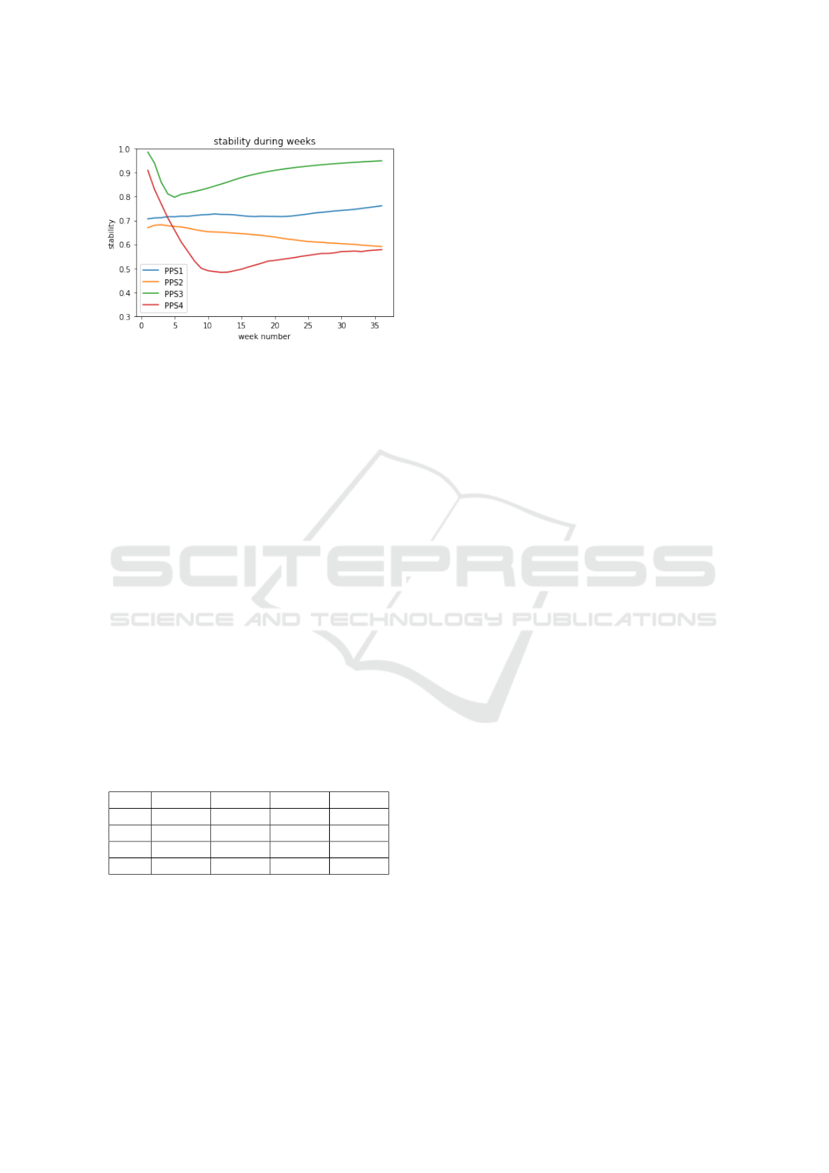
Figure 3: Comparing PPS
1
V, PPS
2
, PPS
3
and PPS
4
in
terms of temporal stability.
The stability of PPS
1
increases slightly over time. It
is at ≈ 70% and ≈ 76% respectively at the first and
last prediction weeks. While the stability of PPS
2
is
decreasing over the weeks. It started with a value of
≈ 64% and ended with ≈ 59%.
Both systems PPS
3
and PPS
4
start with high sta-
bility values ( ≈ 100% and ≈ 92% respectively). This
can be explained by the dominance of the class C
3
,
since at the beginning all learners are assigned to this
class by default. However, these high values decrease
rapidly over the following weeks. For PPS
3
, around
the week 4, it starts to correctly assign each learner to
the suitable class among C
1
, C
2
and C
3
. Then, from
week 5, the stability of PPS
3
increases continuously
and reaches a rate of ≈ 96% at the last prediction
time. For PPS
4
, the shape of the curve is identical
to this of PPS
3
with a downward shift. Until week
13, the overall stability decreases, then from week 14,
it starts to increase again to reach ≈ 57%. We notice
either a partial or a total drop in stability for the sys-
tems PPS
2
, PPS
3
and PPS
4
. Although the stability
of PPS
1
has never decreased over time, PPS
3
remains
the most stable.
Table 3: Stability Measurements.
PPS
1
PPS
2
PPS
3
PPS4
C
1
92.26% 89.12% 58.79% 18.24%
C
2
11.36% 0% 35.85% 0%
C
3
27.56% 0% 47.70% 39.86%
D
test
72.72% 65.12% 88.10% 48.48%
Yet, stability and accuracy are proportional, how-
ever, from the accuracy graphs of PPS
2
and PPS
4
, we
cannot conclude on the effectiveness of the systems in
maintaining correct prediction sequences over time.
6 THREATS TO VALIDITY
The current work presents some limitations that we
tried to mitigate when possible: i) the earliness algo-
rithm returns a single value which corresponds to the
mean of the first correct predictions. However, a high
associated HM is partially reliable as the accuracy of
the system may decrease after the identified earliness.
We intend to consider several earliness points with
respect to the one returned by our algorithm. The
objective is to study the variations of the HM mea-
sures between these earliness points. ii) in this work,
we have adopted a weekly-basis prediction approach.
However, we believe that the proposed indicators can
be also used to define the appropriate temporal gran-
ularity that provides better prediction results. iii) in
the frame of this work, we only considered classifica-
tion problems. To prove the generic use of our indica-
tors, we aim to apply them on other systems that use
regression-based analytical models.
7 CONCLUSION AND
PERSPECTIVES
In this paper, we introduced time-dependent indica-
tors, namely the earliness and stability to assess PPS
used in online distance education. Further, a trade-off
between the earliness and accuracy is important to as-
sess the ability of a PPS to predict learners at-risk of
failure. The use of HM measure serves to illustrate
this balance. The new indicators along with the accu-
racy are used to compare four different PPS. The ex-
perimental results prove that the accuracy is not suffi-
cient to evaluate a PPS within a context of time-series
data. The experimental results show that the HM mea-
sure is relevant in identifying the earliest and accurate
system and that the stability is more pertinent when
the whole test dataset is considered. Further, a system
is considered better when its stability increases over
time.
As perspectives for this work, we intend to im-
prove the proposed earliness algorithm so that it re-
turns a set of different earliness values. Such a re-
sult will enable us to study more deeply the behavior
of the PPS. In addition, our next goal is to study the
trade-off between the stability and earliness indicators
and conclude on the relation between both of them.
REFERENCES
Adnan, M., Habib, A., Ashraf, J., Mussadiq, S., Raza,
A. A., Abid, M., Bashir, M., and Khan, S. U. (2021).
Assess Performance Prediction Systems: Beyond Precision Indicators
495

Predicting at-risk students at different percentages of
course length for early intervention using machine
learning models. IEEE Access, 9:7519–7539.
Ba
˜
neres, D., Rodr
´
ıguez, M. E., Guerrero-Rold
´
an, A. E., and
Karadeniz, A. (2020). An early warning system to de-
tect at-risk students in online higher education. Ap-
plied Sciences, 10(13):4427.
Ben Soussia, A., Roussanaly, A., and Boyer, A. (2021).
An in-depth methodology to predict at-risk learners.
In European Conference on Technology Enhanced
Learning, pages 193–206. Springer.
Chui, K. T., Fung, D. C. L., Lytras, M. D., and Lam, T. M.
(2020). Predicting at-risk university students in a vir-
tual learning environment via a machine learning al-
gorithm. Computers in Human Behavior, 107:105584.
Figueroa-Ca
˜
nas, J. and Sancho-Vinuesa, T. (2020). Early
prediction of dropout and final exam performance in
an online statistics course. IEEE Revista Iberoameri-
cana de Tecnologias del Aprendizaje, 15(2):86–94.
Hlosta, M., Zdrahal, Z., and Zendulka, J. (2017).
Ouroboros: early identification of at-risk students
without models based on legacy data. In Proceed-
ings of the seventh international learning analytics &
knowledge conference, pages 6–15.
Hu, Y.-H., Lo, C.-L., and Shih, S.-P. (2014). Develop-
ing early warning systems to predict students’ online
learning performance. Computers in Human Behav-
ior, 36:469–478.
Iqbal, Z., Qadir, J., Mian, A. N., and Kamiran, F. (2017).
Machine learning based student grade prediction: A
case study. arXiv preprint arXiv:1708.08744.
Karalar, H., Kapucu, C., and G
¨
ur
¨
uler, H. (2021). Predict-
ing students at risk of academic failure using ensem-
ble model during pandemic in a distance learning sys-
tem. International Journal of Educational Technology
in Higher Education, 18(1):1–18.
Lee, S. and Chung, J. Y. (2019). The machine learning-
based dropout early warning system for improving the
performance of dropout prediction. Applied Sciences,
9(15):3093.
Philipp, M., Rusch, T., Hornik, K., and Strobl, C. (2018).
Measuring the stability of results from supervised
statistical learning. Journal of Computational and
Graphical Statistics, 27(4):685–700.
Sch
¨
afer, P. and Leser, U. (2020). Teaser: early and accurate
time series classification. Data mining and knowledge
discovery, 34(5):1336–1362.
Teinemaa, I., Dumas, M., Leontjeva, A., and Maggi, F. M.
(2018). Temporal stability in predictive process mon-
itoring. Data Mining and Knowledge Discovery,
32(5):1306–1338.
Wang, W., Yu, H., and Miao, C. (2017). Deep model for
dropout prediction in moocs. In Proceedings of the
2nd international conference on crowd science and
engineering, pages 26–32.
Wolff, A., Zdrahal, Z., Herrmannova, D., Kuzilek, J., and
Hlosta, M. (2014). Developing predictive models for
early detection of at-risk students on distance learning
modules.
Zhang, W., Huang, X., Wang, S., Shu, J., Liu, H., and Chen,
H. (2017). Student performance prediction via on-
line learning behavior analytics. In 2017 International
Symposium on Educational Technology (ISET), pages
153–157. IEEE.
A2E 2022 - Special Session on Analytics in Educational Environments
496