Optimal Prediction of Tessarine Signals from Multi-sensor Uncertain

Observations under T

-Properness Conditions

Jos

e Domingo Jim

enez-L

opez

, Rosa Mar

ıa Fern

andez-Alcal

, Jes

us Navarro-Moreno

and Juan Carlos Ruiz-Molina

Department of Statistics and Operations Research, University of Ja

en, Paraje Las Lagunillas s/n, 23071 Ja

en, Spain

Keywords:

Multisensor Systems, Optimal Prediction, Tessarine Signal Processing, T

-Properness Conditions, Uncertain

Observations.

Abstract:

In this paper, the optimal one-stage prediction problem of tessarine signals from multi-sensor uncertain ob-

servations is approached. At each instant of time, there exists a non-null probability that the observation

tessarine component coming from each sensor, contains the corresponding signal component, or only noise.

To model the uncertainty, multiplicative noises modeled by Bernoulli random variables are included in the

observation equations. Under correlation hypotheses between the signal and observation additive noises, a

recursive algorithm to calculate the optimal least-squares linear predictor of the signal and its mean-squared

error is proposed, derived by using an innovation approach. The theoretical results are illustrated by means

of a numerical simulation example, in which the performance of the proposed estimator is evaluated under

different uncertainty probabilities.

1 INTRODUCTION

Traditionally, the real and complex domains have con-

stituted the framework to model random signals in dy-

namical systems. However, in the last two decades,

there has been an increasing interest in the scientiﬁc

community to study higher-dimensional spaces, due

to the fact that they are more appropriate to model a

great number of physical phenomena. As an exam-

ple, hypercomplex signals are used to model biomed-

ical phenomena (Abbasi-Kesbi and Nikfarjam, 2018;

Ajdaroski et al., 2022), avionics, as unmanned aerial

vehicles (Zheng et al., 2020; Qu and Yi, 2022), neu-

ral networks (Bayro-Corrochano et al., 2021; Wei

et al., 2022), acoustic applications (Ortolani et al.,

2016; Celsi et al., 2020), communication (Grakhova

et al., 2019; Ahmad et al., 2021), image processing

(Augereau and Carr

e, 2017; Yang et al., 2022), etc.

Recently, in real signal processing, estimation

problems have been approached from observations

provided by multiple sensors. The fact that the sig-

nal is estimated from multisensor observations, yields

https://orcid.org/0000-0003-1263-5508

https://orcid.org/0000-0002-3329-6624

https://orcid.org/0000-0002-8417-8505

https://orcid.org/0000-0002-3128-8030

better estimates than those traditionally obtained by

a single sensor, since more observations are avail-

able, and also it is possible to avoid the negative ef-

fect in the estimation caused by observations from

faulty sensors. In the real domain, there exists a wide-

ranging literature on signal processing from multisen-

sor observations affected by different uncertainties,

that frequently occur in the transmission problems.

For example, assuming missing or intermittent mea-

surements, the estimation problem has been solved in

the real ﬁeld by using the centralized fusion method

(Liu et al., 2017) and the distributed fusion proce-

dure (Lin and Sun, 2016). Another common situation

consists of considering that the observations may be

updated or delayed at each instant of time (Linares-

erez et al., 2009; Liang et al., 2011). Both uncertain-

ties can be also simultaneously studied (Zhang et al.,

2021), or even include multiple packet dropouts, in

which case the last observation successfully transmit-

ted is considered if the real observation is not avail-

able (Ma and Sun, 2013).

So, the need to extend the obtained results on the

real signal estimation problems to the hypercomplex

domains arises. However, this generalization is not

an immediate extension from the real vectorial case,

due to the fact that the hypercomplex algebras lose

important properties of the algebraic operations in the

Jiménez-López, J., Fernández-Alcalá, R., Navarro-Moreno, J. and Ruiz-Molina, J.

Optimal Prediction of Tessarine Signals from Multi-sensor Uncertain Observations under Tk-Properness Conditions.

DOI: 10.5220/0011124200003271

In Proceedings of the 19th International Conference on Informatics in Control, Automation and Robotics (ICINCO 2022), pages 577-584

ISBN: 978-989-758-585-2; ISSN: 2184-2809

577

real ﬁeld. Moreover, under certain properties of the

processes involved in the system model, a reduction

in the dimension of the model is obtained, fact that it

can not be considered in the real ﬁeld. Most of the es-

timation problems in the hypercomplex domains have

been studied in the quaternion space, due to the fact

that it has a Hilbert space structure, although the prod-

uct is not commutative. In the quaternion domain, the

widely linear (WL) estimation problem, that is, that

means to consider the signal and its three involutions,

has been solved under different uncertainty hypothe-

ses (Jim

enez-L

opez et al., 2017; Fern

andez-Alcal

et al., 2020). Assuming C

-property conditions, the

processing is called semi-widely linear (SWL) one,

and it considers the signal and the involution over the

pure unit quaternion (Navarro-Moreno et al., 2019).

The signal estimation problems in the tessarine

domain have been less studied since it is not a Hilbert

space. Recently, a metric has been deﬁned in the

tessarine domain that satisﬁes the necessary proper-

ties to guarantee the existence and uniqueness of the

least-squares linear estimator (Navarro-Moreno et al.,

2020). Moreover, from analogy with the quaternion

domain, T

and T

-properness conditions have been

deﬁned in the tessarine domain, getting so a reduc-

tion in the dimension of the model (Navarro-Moreno

et al., 2020; Navarro-Moreno and Ruiz-Molina, 2021;

Fern

andez-Alcal

a et al., 2021).

In this paper, the least-squares linear one-stage

prediction problem is approached by considering a

state-pace model with uncertain observations pro-

vided by multiple sensors. Under correlation hy-

potheses on the additive noises and T

-properness

conditions, a recursive prediction algorithm is pro-

posed. A numerical simulation example illustrates the

theoretical results obtained.

2 MODEL FORMULATION

In this section, the tessarine state-space model is pre-

sented by means of the signal and multi-sensor ob-

servation equations. Notation R and T will be used

to the set of real numbers and tessarine ﬁeld, respec-

tively. Moreover, unless otherwise stated, all the ran-

dom variables are assumed to have zero-mean.

Let us consider a n-dimensional tessarine random

signal vector x(t) ∈ T

, which is given as follows

x(t) = x

(t) + ηx

(t) + η

′

(t) + η

′′

(t), (1)

where x

(t) ∈ R

, for ν = r, η,η

′

,η

′′

, are n-

dimensional real random signal vector and {η, η

′

,η

′′

}

denote the imaginary units satisfying the following

identities:

ηη

′

= η

′′

, η

′

′′

= η, η

′′

η = −η

′

= −η

′ 2

= η

′′ 2

= −1.

Let us assume the following state equation for x(t):

x(t + 1) = F

(t)x(t) + F

(t)x

∗

(t) + F

(t)x

(t)

+ F

(t)x

′′

(t) + u(t), t ≥ 0,

(2)

where F

(t) ∈ T

n×n

, for i = 1, . . . , 4, are tessarine de-

terministic matrices of dimension n × n, x

(t), for

ν = ∗,η,η

′′

, are the corresponding conjugations of the

tessarine signal in (1), deﬁned as follows

∗

(t) = x

(t) − ηx

(t) + η

′

(t) − η

′′

(t),

(t) = x

(t) + ηx

(t) − η

′

(t) − η

′′

(t),

′′

(t) = x

(t) − ηx

(t) − η

′

(t) + η

′′

(t),

and u(t) ∈ T

is a tessarine white noise with pseudo

variance matrix Q(t).

Consider that the signal x(t) is estimated from

the observations provided by m sensors, denoted by

(i)

(t) ∈ T

, for i = 1, . . . , m, satisfying the following

observation equation:

(i)

(t) = γ

(i)

(t) ◦ x

(t) + ηγ

(i)

(t) ◦ x

(t)

+ η

′

(i)

′

(t) ◦ x

′

(t) + η

′′

(i)

′′

(t) ◦ x

′′

(t)

+ v

(i)

(t), t ≥ 1,

(3)

where ◦ denotes the Hadamard product, and v

(i)

(t) ∈

is a tessarine white noise with pseudo variance ma-

trix R

(i)

(t). Moreover, for each sensor i = 1, . . . , m,

and ν = r, η, η

′

,η

′′

, γ

(i)

(t) is a n-dimensional vec-

tor whose components, γ

(i)

j,ν

(t), are Bernoulli ran-

dom variables with known parameters p

(i)

j,ν

(t). So, if

(i)

ν, j

(t) = 1, then the component y

(i)

j,ν

(t) contains sig-

nal and noise, and in contrast, if it takes the value 0,

then the corresponding observation component con-

tains only noise.

Let us assume that for each sensor i = 1,...,m,

and ν = r, η, η

′

,η

′′

, the Bernoulli random variables in

(i)

(t) are independent of those in γ

(i)

(s), for s ̸= t.

Moreover, v

(i)

(t) is independent of v

( j)

(t) for i, j =

1,...,m, with i ̸= j. The additive noises are corre-

lated, E

u(t)v

(i)

(t)

= S

(i)

(t) (where H denotes the

Hermitian operator), and P

denotes the pseudo vari-

ance matrix of the signal at the initial state. Finally,

let us consider that x(0) and the noises {u(t);t ≥ 0},

(i)

(t);t ≥ 1} and {γ

(i)

(t);t ≥ 1}, for ν = r, η, η

′

,η

′′

i = 1, . . . , m, are mutually independent.

From equations (2) and (3), the following aug-

mented state-space model can be obtained

x(t + 1) =

Φ(t)

x(t) +

u(t), t ≥ 0,

(i)

(t) = D

(i)

(t)

x(t) +

(i)

(t), t ≥ 1,

(4)

ICINCO 2022 - 19th International Conference on Informatics in Control, Automation and Robotics

578

where

a(t) =

(t),a

∗

(t),a

′′

(t)

, for a =

x,u,y

(i)

, where T denotes the transpose operator,

Φ(t) =







(t) F

(t)

∗

(t) F

∗

(t) F

∗

(t) F

∗

(t)

(t) F

(t)

′′

(t) F

′′

(t) F

′′

(t) F

′′

(t)







(i)

(t) = T

diag(γ

(i)

(t))T

with γ

(i)

(t) =

(i)

(t),γ

(i)

(t),γ

(i)

′

(t),γ

(i)

′′

(t)

diag(γ

(i)

(t)) denotes a diagonal matrix with

the elements γ

(i)

(t) on the main diagonal, and

A ⊗ I

, with

A =







1 η η

′

′′

1 −η η

′

−η

′′

1 η −η

′

−η

′′

1 −η −η

′

′′







and I

the identity matrix of dimension n.

The pseudo variance matrices of the additive

noises

u(t) and

(i)

(t) in (4) are denoted by

Q(t) and

(i)

(t), respectively. Moreover, E

u(t)

(i)

(s)

(i)

(t)δ

t,s

, where δ denotes the Kronecker delta func-

tion, and E [

x(0)

(0)] =

2.1 T

-Properness Conditions

The T

-properness concept, for k = 1, 2, has been

recently deﬁned (Navarro-Moreno et al., 2020;

Navarro-Moreno and Ruiz-Molina, 2021), and it is

related with the fact that some of the pseudo corre-

lation functions of the signal with its conjugations

vanish. This property reduces the dimension of the

augmented state model and, hence, the computational

burden necessary to carry out the estimations de-

creases.

The pseudo autocorrelation function of the ran-

dom signal x(t) ∈ T

is deﬁned as Γ

(t,s) =

E [x(t)x

(s)], ∀t,s ∈ Z (Z denotes the set of integer),

and the pseudo cross correlation function of the ran-

dom signals x(t) ∈ T

and y(t) ∈ T

is deﬁned as

(t,s) = E [x(t)y

(s)], ∀t,s ∈ Z.

A random signal x(t) ∈ T

is said to be:

· T

-proper, if, and only if,

∗

(t,s) = Γ

′′

(t,s) = 0,

· T

-proper, if, and only if,

(t,s) = Γ

′′

(t,s) = 0,

for all t, s ∈ Z. Similarly, two random signals x(t) ∈

and y(t) ∈ T

are:

· cross T

-proper, if, and only if,

∗

(t,s) = Γ

′′

(t,s) = 0,

· cross T

-proper, if, and only if,

(t,s) = Γ

′′

(t,s) = 0,

for all t, s ∈ Z. Finally, x(t) and y(t) are jointly T

proper (respectively, jointly T

-proper) if, and only if,

they are T

-proper (respectively, T

-proper) and cross

-proper (respectively, cross T

-proper).

For the model described in equation (4), the fol-

lowing T

-properness conditions can be established:

1. If x(0) and u(t) are T

-proper, and

Φ(t) is a block

diagonal matrix of the form

Φ(t) = diag



(t),F

∗

(t),F

′′

(t)



then x(t) is T

-proper. If additionally p

(i)

j,ν

(t) ≡

(i)

(t), for all i = 1, . . . , m, j = 1, . . . , n, ν =

r, η, η

′

,η

′′

,t ∈ Z, v

(i)

(t) is T

-proper, and u(t) and

(i)

(t) are cross T

-proper, then x(t) and y

(i)

(t)

are jointly T

-proper. Under these conditions,

(i)

(t) = E

(i)

(t)

= I

⊗Π

(i)

(t), i = 1, . . . , m,

with

(i)

(t) = diag



(i)

1,r

(t),..., p

(i)

n,r

(t)



, i = 1, . . . , m.

(5)

2. Analogously, if x(0) and u(t) are T

-proper, and

Φ(t) is a block diagonal matrix of the form

Φ(t) = diag



(t),Φ

(t)



with

(t) =



(t) F

(t)

∗

(t) F

∗

(t)



, (6)

then x(t) is T

-proper. If additionally p

(i)

j,r

(t) =

(i)

j,η

(t) and p

(i)

j,η

′

(t) = p

(i)

j,η

′′

(t), i = 1, . . . , m, j =

1,...,n,t ∈ Z, v

(i)

(t) is T

-proper, and u(t) and

(i)

(t) are cross T

-proper, then x(t) and y

(i)

(t)

are jointly T

-proper. In that case,

(i)

(t) = diag



(i)

(t),Π

(i)

(t)



, i = 1, . . . , m,

with

(i)

(t) =

(i)

(t) Π

(i)

−

(t)

(i)

−

(t) Π

(i)

(t)

, i = 1, . . . , m,

(7)

Optimal Prediction of Tessarine Signals from Multi-sensor Uncertain Observations under Tk-Properness Conditions

579

and

(i)

(t) = diag



(i)

1,r

(t) + p

(i)

1,η

′

(t),...

..., p

(i)

n,r

(t) + p

(i)

n,η

′

(t)



(i)

−

(t) = diag



(i)

1,r

(t) − p

(i)

1,η

′

(t),...

..., p

(i)

n,r

(t) − p

(i)

n,η

′

(t)



for i = 1, . . . , m.

2.2 T

-Proper System Model

Under T

-properness conditions, a reduction in the di-

mension of the system model described in (4) is ob-

tained. Next the new situations are described.

· In the T

-proper scenario. The processes

x(t),

u(t)

(i)

(t),

(i)

(t) and

Φ(t), are substituted

by x

(t) ≜ x(t), u

(t) ≜ u(t), y

(i)

(t) ≜ y

(i)

(t),

(i)

(t) ≜ v

(i)

(t) and Φ

(t) ≜ F

(t). The pseudo

variance and cross-covariance matrices of the

noises are given by Q

(t) = Q(t), R

(i)

(t) = R

(i)

(t)

and S

(i)

(t) = S

(i)

(t). The observation equation in

(4) is now expressed as follows

(i)

(t) = D

(i)

(t)

x(t) + v

(i)

(t), t ≥ 1

where

(i)

(t) = T

diag



(i)

(t)



, i = 1, . . . , m,

with



1 η η

′

′′



⊗ I

. (8)

Then,

(i)

(t) = E

(i)

(t)

(i)

(t),0

n×3n

, (9)

where Π

(i)

(t) is given in (5), and 0

n×3n

represents

the n × 3n zero matrix.

· In the T

-proper scenario. Now the pro-

cesses

x(t),

u(t)

(i)

(t),

(i)

(t) and

Φ(t), are

substituted by x

(t) ≜ [x(t), x

(t)]

, u

(t) ≜

[u(t),u

(t)]

, z

(i)

(t) ≜

(i)

(t),z

(i)

(t)

, v

(i)

(t) ≜

(i)

(t),v

(i)

(t)

and Φ

(t) (deﬁned in (6)). The

pseudo variance and cross-covariance matrices

of the noises are denoted by Q

(t), R

(i)

(t) and

(i)

(t). The reduced observation equation is now

expressed as

(i)

(t) = D

(i)

(t)

x(t) + v

(i)

(t), t ≥ 1

where

(i)

(t) = T

diag



(i)

(t)



, i = 1, . . . , m,

with



1 η η

′

′′

1 −η η

′

−η

′′



⊗ I

, (10)

and

(i)

(t) = E

(i)

(t)

(i)

(t),0

2n×2n

, (11)

where Π

(i)

(t) is given in (7).

3 OPTIMAL PREDICTION

ALGORITHM

In this section, the optimal one-stage prediction prob-

lem of the signal x(t) from all the observations

provided by the m sensors is addressed, under T

properness conditions. So, denoting by

⃗

y(t) the vec-

tor formed by the observations from all the sensors,

that is,

⃗

y(t) =

(1)

(t),...,

(m)

(t)

, our aim is to

obtain recursive formulas to obtain the optimal least-

squares linear estimator of the signal x(t) from the ob-

servations until previous instant,

{

⃗

y(1),...,

⃗

y(t − 1)

}

The observation equation is now expressed as follows

⃗

y(t) =

⃗

(t)Λ

x(t) +

⃗

v(t), t ≥ 1

where

⃗

(t) = ϒ

diag



⃗

(t)



, with ϒ

= I

⊗T

and

⃗

(t) =



(1)

(t),...,γ

(m)

(t)



, Λ

= 1

⊗ I

where 1

denotes the m × 1 vector with all its el-

ements 1, and

⃗

v(t) =

(1)

(t),...,

(m)

(t)

. The

pseudo variance and cross-covariance matrices of the

additive noises are given by:

⃗

R(t) = E [

⃗

v(t)

⃗

(t)] =

diag



(1)

(t),...,

(m)

(t)



, E [

u(t)

⃗

(s)] =

⃗

S(t)δ

with

⃗

S(t) =

(1)

(t),...,

(m)

(t)

However, under T

-properness conditions, for k =

1,2, a reduction of the dimension in the state-space

model is obtained; so, assuming this property, the ob-

servation equation is given as follows

(t) =

⃗

(t)Λ

x(t) +

⃗

v(t), t ≥ 1,

(12)

where

⃗

(t) = ϒ

diag(

⃗

(t))ϒ

, with ϒ

= I

⊗ T

and T

for k = 1, 2 are given in (8) and (10), respec-

tively. Moreover,

⃗

(t) =E

⃗

(t)

=diag



(1)

(t),...,Π

(m)

(t)



ICINCO 2022 - 19th International Conference on Informatics in Control, Automation and Robotics

580

with Π

(i)

(t), for i = 1, . . . , m, given in (9) and (11) for

k = 1, 2, respectively.

Next result proposes a recursive algorithm to

obtain the optimal one-stage predictor under T

properness conditions, denoted by

(t|t − 1), as

well as its mean squared error.

Theorem 1. Under T

-properness conditions, for k =

1,2, in the model described by equations (2) and (12)

and the hypotheses assumed, the optimal one-stage

predictor,

(t|t − 1), is obtained by extracting the

ﬁrst n components of

(t|t − 1), which is recursively

calculated as follows

(t|t − 1) =Φ

(t − 1)

(t − 1|t − 1)

+ H

(t − 1)ε

(t − 1), t ≥ 2,

where

(t − 1|t − 1) satisﬁes this formula

(t − 1|t − 1) =

(t − 1|t − 2)

+ L

(t − 1)ε

(t − 1), t ≥ 2,

with initial conditions

(1|0) =

(0|0) = 0

The matrices H

(t) and L

(t) are calculated as:

(t) = S

(t)Ω

−1

(t) and L

(t) = Θ

(t)Ω

−1

(t) ,

where S

(t) = [S

(1)

(t),...,S

(m)

(t)], with S

(i)

(t), for

i = 1, . . . , m, deﬁned in Section 2.2.

The innovations, ε

(t), are obtained as follows

(t) = y

(t) − Π

(t)Λ

(t|t − 1), t ≥ 1,

where Λ

= 1

⊗ I

, and Π

(t) =

diag



(1)

(t),...,Π

(m)

(t)



, with Π

(i)

(t) for k = 1, 2,

are given in (5) and (7), respectively.

The matrices Θ

(t) satisfy this relation

(t) = P

(t|t − 1)Λ

(t), t ≥ 2;

(1) = 1

⊗ D

(1)Π

(1),

with

(1) =



kn×(4−k)n





Φ(0)

P(0)

(0) +

Q(0)





kn×(4−k)n



The pseudo covariance matrix of the innovations,

Ω

(t), is obtained from this expression

Ω

(t) = ϒ



Cov(

⃗

(t)) ◦



D(t)Λ



+ Π

(t)Ξ

(t|t − 1)Ξ

(t)

+ R

(t), t ≥ 2,

Ω

(1) = I

⊗ Π

(1)D

(1)Π

(1) + R

(1),

where

D(t) can be recursively calculated by this for-

mula

D(t) =

Φ(t − 1)

D(t − 1)

(t − 1) +

Q(t − 1), t ≥ 1,

D(0) =

and R

(t) = diag



(1)

(t),...,R

(m)

(t)



, with R

(i)

(t),

for i = 1, . . . , m, deﬁned in Section 2.2.

Finally, the prediction error covariance matrices,

(t|t − 1), are calculated from P

(t|t − 1), which

satisfy the following equation

(t|t − 1) = Φ

(t − 1)P

(t − 1|t − 1)Φ

(t − 1)

− Φ

(t − 1)Θ

(t − 1)H

(t − 1)

− H

(t − 1)Θ

(t − 1)Φ

(t − 1)

− H

(t − 1)Ω

(t − 1)H

(t − 1)

+ Q

(t − 1), t ≥ 1

where P

(t −1|t −1) can be recursively obtained from

this relation

(t − 1|t − 1) = P

(t − 1|t − 2)

− Θ

(t − 1)Ω

−1

(t − 1)

× Θ

(t − 1), t ≥ 1,

with initial conditions

(0|0) =



kn×(4−k)n





kn×(4−k)n



and P

(1|0) = D

(1).

4 NUMERICAL EXAMPLE

Our goal in this section is to illustrate the performance

of the proposed estimator by considering the follow-

ing tessarine state-space model with ﬁve sensors:

x(t + 1) = f x(t) + u(t), t ≥ 0,

(i)

(t) = γ

(i)

(t)x

(t) + ηγ

(i)

(t)x

(t) + η

′

(i)

′

(t)x

′

(t)

+ η

′′

(i)

′′

(t)x

′′

(t) + v

(i)

(t), t ≥ 1,

for i = 1, . . . , 5,, where f = 0.9 + 0.3η + 0.1η

′

0.1η

′′

∈ T,

(i)

(t);t ≥ 1

ν=r,η,η

′

,η

′′

are sequences of

Bernoulli random variables with parameters p

(i)

(t),

and u(t) and v

(i)

(t) are tessarine Gaussian noises.

Moreover, the real covariance matrix of u(t) is

given as follows

(t)u

(s)







0.9 0 b 0

0 a 0 b

b 0 0.9 0

0 b 0 a







, (13)

with u

(t) =



(t),u

′

(t),u

′′

(t)



The additive observation noises, v

(i)

(t), are de-

ﬁned as

(i)

(t) = α

u(t) + w

(i)

(t),

Optimal Prediction of Tessarine Signals from Multi-sensor Uncertain Observations under Tk-Properness Conditions

581

with α

= 0.5,α

= 0.3,α

= 0.4,α

= 0.6,α

= 0.2,

and w

(i)

(t) tessarine zero-mean white Gaussian noises

with real covariance matrices

(i)

(t)w

(i)

(s)

= diag (β

,β

)δ

with w

(i)

(t) =

(i)

(t),w

(i)

(t),w

(i)

′

(t),w

(i)

′′

(t)

and

= 3, β

= 7, β

= 15, β

= 21, β

= 25.

It is also assumed that the variance matrix of the

real initial state is given as follows

(0)x

(0)







c 0 d 0

0 4 0 d

d 0 c 0

0 d 0 4







, (14)

with x

(0) =



(0),x

′

(0),x

′′

(0)



Finally, the mutual independence hypothesis be-

tween the initial state and the multiplicative and addi-

tive noises is also considered.

The performance of the proposed estimator is

analysed in both T

and T

-proper scenarios by tak-

ing different values of the Bernoulli parameters, as-

suming that these are constant in time, that is, for each

i = 1, . . . , 5, ν = r, η, η

′

,η

′′

, p

(i)

(t) = p

(i)

, for all t.

4.1 T

-Proper Case

In order to guarantee the T

-properness conditions, let

us consider a = 0.9, b = 0.3 in (13), and c = 4, d =

−2.5 in (14). Moreover, p

(i)

= p

(i)

, for ν = r, η, η

′

′′

Under these assumptions, x(t) and y

(i)

(t), i = 1, . . . , 5

are jointly T

-proper.

Firstly, in order to show the effectiveness of the

proposed estimator in comparison with the one-stage

predictor obtained at each sensor, the error variances

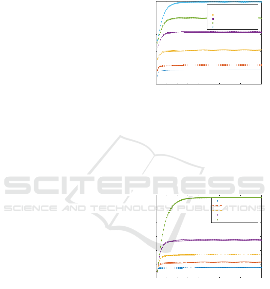
are computed in Figure 1 for the following values of

the Bernoulli parameters: Sensor 1, p

(1)

= 0.9; Sen-

sor 2, p

(2)

= 0.7; Sensor 3, p

(3)

= 0.5; Sensor 4,

(4)

= 0.3; Sensor 5, p

(5)

= 0.1. It is observed that

the performance of the proposed estimator, that uses

the observations provided for all the sensors, is bet-

ter than any of the estimators obtained from the ob-

servations of each sensor. Note that the probability

that the observation at each sensor contains the sig-

nal decreases from Sensor 1 to 5, that is, at Sensor 1,

it is more probable that the observation contains sig-

nal and noise, but the opposite happens at Sensor 5,

it is more probable that the observation contains only

noise. As it is observed, as this probability decreases,

from Sensor 1 to 5, the error variances increases, and

then the accuracy of the estimator is worse.

Now, in order to show the performance of the pro-

posed estimator with regards to the Bernoulli proba-

bilities, the error variances are computed for different

0 10 20 30 40 50 60 70 80 90 100

Prediction error variance

Error variances for all sensors

Error variances for Sensor 1

Error variances for Sensor 2

Error variances for Sensor 3

Error variances for Sensor 4

Error variances for Sensor 5

Figure 1: Prediction error variances for the proposed es-

timator and for the one obtained from the observations at

Sensor i, for i = 1,.. . ,5.

values of them. Speciﬁcally, the same probability has

been taken in all the sensors, decreasing from 0.9 to

0.1, that is, the following situations have been con-

sidered: p

(i)

= 0.9,∀i; p

(i)

= 0.7,∀i; p

(i)

= 0.5,∀i;

(i)

= 0.3, ∀i and p

(i)

= 0.1, ∀i. As before, it is ob-

served that as the Bernoulli probabilities of all the

sensors decrease, which means that it is more prob-

able that the observations contain more noise and less

signal, the error variances increase and hence, the es-

timations are worse.

0 10 20 30 40 50 60 70 80 90 100

Prediction error variance

Error variances for p

(i)

=0.9

Error variances for p

(i)

=0.7

Error variances for p

(i)

=0.5

Error variances for p

(i)

=0.3

Error variances for p

(i)

=0.1

Figure 2: Prediction error variances for the proposed esti-

mator taking the same probability in all the sensors.

4.2 T

-Proper Case

Consider the values a = 0.6, b = 0.3 in (13), and c =

3, d = −2.5 in (14), and also, p

(i)

= p

(i)

and p

(i)

′

(i)

′′

. So, x(t) and y

(i)

(t), i = 1, . . . , 5 are jointly T

proper.

Now, under T

-properness conditions, analogous

situations to Figures 1 and 2, have been illustrated

ICINCO 2022 - 19th International Conference on Informatics in Control, Automation and Robotics

582

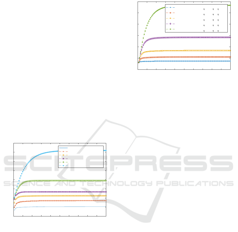
in Figures 3 and 4, respectively. For this purpose,

in Figure 3, the prediction error variances for the

proposed estimator which uses the observations of

all the sensors, as well as for the estimator at each

sensor, are shown by taking the following proba-

bility values: Sensor 1,



(1)

, p

(1)

′



= (0.9,0.8);

Sensor 2,



(2)

, p

(2)

′



= (0.7, 0.6); Sensor 3,



(3)

, p

(3)

′



= (0.5, 0.4); Sensor 4,



(4)

, p

(4)

′



(0.3,0.2); Sensor 5,



(5)

, p

(5)

′



= (0.1, 0.05).

And, in Figure 4, the prediction error variances

for the proposed estimator have been displayed by

considering the same probability in all the sensors

at these situations:



(i)

, p

(i)

′



= (0.9, 0.8), ∀i;



(i)

, p

(i)

′



= (0.7,0.6),∀i;



(i)

, p

(i)

′



(0.5,0.4),∀i;



(i)

, p

(i)

′



= (0.3, 0.2), ∀i; and



(i)

, p

(i)

′



= (0.1,0.05),∀i. Analogous considera-

tions to that of Figures 1 and 2, in the T

-proper case,

are deduced.

0 10 20 30 40 50 60 70 80 90 100

Prediction error variance

Error variances for all sensors

Error variances for Sensor 1

Error variances for Sensor 2

Error variances for Sensor 3

Error variances for Sensor 4

Error variances for Sensor 5

Figure 3: Prediction error variances for the proposed es-

timator and for the one obtained from the observations at

Sensor i, for i = 1,.. . ,5.

5 CONCLUSIONS

Recently, the scientiﬁc community has shown an in-

creasing interest in the use of hypercomplex algebras

to model many experimental phenomena, as well as

in assuming that the observations of the signal to be

estimated are provided by multiple sensors. The ﬁrst

aim is due to the fact that the hypercomplex domains

are more appropriate than the real ﬁeld to describe

a great amount of physical variables and also, un-

der certain properness conditions, a reduction in the

computational burden involved in the estimation al-

0 10 20 30 40 50 60 70 80 90 100

Prediction error variance

Error variances for p

(i)

=0.9,p

(i)

´´

=0.8

Error variances for p

(i)

=0.7,p

(i)

´´

=0.6

Error variances for p

(i)

=0.5,p

(i)

´´

=0.4

Error variances for p

(i)

=0.3,p

(i)

´´

=0.2

Error variances for p

(i)

=0.1,p

(i)

´´

=0.05

Figure 4: Prediction error variances for the proposed esti-

mator taking the same probability in all the sensors.

gorithms is attained. The last goal is due to the fact

that the use of multisensor observations yields better

estimations.

The generalization of the signal processing results

obtained in the real ﬁeld to the hypercomplex domain

is not immediate. Some of the main properties of the

algebraic operations in the real ﬁeld are not valid in

the hypercomplex domains. Until now, most of the

results obtained on hypercomplex signal estimation

have been approached in the quaternion domain, since

it has a Hilbert space structure. However, commuta-

tive hypercomplex algebras such as tessarines, pro-

vide a suitable structure to extend the main results

in the real and complex ﬁeld to this one. Although

the tessarine domain is not a Hilbert space, a norm

has been recently deﬁned to guarantee the existence

and uniqueness of the optimal least squares linear es-

timator (Navarro-Moreno et al., 2020). From this last

result, the tessarine signal estimation problem is cur-

rently an important research object.

ACKNOWLEDGEMENTS

This work has been supported in part by I+D+i project

with reference number 1256911, under ‘Programa

Operativo FEDER Andaluc

ıa 2014-2020’, Junta de

Andaluc

ıa, and Project EI-FQM2-2021 of ‘Plan de

Apoyo a la Investigaci

on 2021-2022’ of the Univer-

sity of Ja

en.

REFERENCES

Abbasi-Kesbi, R. and Nikfarjam, A. (2018). A miniature

sensor system for precise hand position monitoring.

IEEE Sensors Journal, 18(6):2577–2584.

Ahmad, Z., Hashim, S., Rokhani, F., Al-Haddad, S., Sali,

Optimal Prediction of Tessarine Signals from Multi-sensor Uncertain Observations under Tk-Properness Conditions

583

A., and Takei, K. (2021). Quaternion model of

higher-order rotating polarization wave modulation

for high data rate m2m lpwan communication. Sen-

sors, 21:383.

Ajdaroski, M., Ashton-Miller, J., Baek, S., Shahshahani,

P., and Esquivel, A. (2022). Testing a quater-

nion conversion method to determine human three-

dimensional tibiofemoral angles during an in vitro

simulated jump landing. Journal of biomechanical en-

gineering, 144(4):041002.

Augereau, B. and Carr

e, P. (2017). Hypercomplex poly-

nomial wavelet-ﬁlter bank transform for color image.

Signal Processing, 136:16–28.

Bayro-Corrochano, E., Solis-Gamboa, S., Altamirano-

Escobedo, G., Lechuga-Gutierres, L., and Lisarraga-

Rodriguez, J. (2021). Quaternion spiking and quater-

nion quantum neural networks: Theory and appli-

cations. International Journal of Neural Systems,

31(2):2050059.

Celsi, M., Scardapane, S., and Comminiello, D. (2020).

Quaternion neural networks for 3d sound source lo-

cation in reverberant environments. In MLSP’2020,

IEEE international Workshop on Machine Learning

for Signal Processing, page 9231809.

Fern

andez-Alcal

a, R. M., Navarro-Moreno, J., Jim

enez-

opez, J. D., and Ruiz-Molina, J. C. (2020). Semi-

widely linear estimation algorithms of quaternion sig-

nals with missing observations and correlated noises.

Journal of the Franklin Institute, 357:3075–3096.

Fern

andez-Alcal

a, R. M., Navarro-Moreno, J., and Ruiz-

Molina, J. C. (2021). T-proper hypercomplex cen-

tralized fusion estimation for randomly multiple sen-

sor delays systems with correlated noises. Sensors,

21(17):5729.

Grakhova, E., Abdrakhmanova, G., Schmidt, S., Vino-

gradova, I., and Sultanov, A. (2019). The quadrature

modulation of quaternion signals for capacity upgrade

of high-speed ﬁber-optic wireless communication sys-

tems. In SPIE - The Society for Optical Engineering,

page 11146.

Jim

enez-L

opez, J. D., Fern

andez-Alcal

a, R. M., Navarro-

Moreno, J., and Ruiz-Molina, J. C. (2017). Widely

linear estimation of quaternion signals with intermit-

tent observations. Signal Processing, 136:92–101.

Liang, J., Shen, B., Dong, H., and Lam, J. (2011). Robust

distributed state estimation for sensor networks with

multiple stochastic communication delays. Interna-

tional Journal of Systems Science, 42(9):1459–1471.

Lin, H. and Sun, S. (2016). Distributed fusion estima-

tor for multi-sensor asynchronous sampling systems

with missing measurements. IET Signal Processing,

10(7):724–731.

Linares-P

erez, J., Carazo, A. H., Caballero-

Aguila, R., and

Jim

enez-L

opez, J. D. (2009). Least-squares linear ﬁl-

tering using observations coming from multiple sen-

sors with one- or two-step random delay. Signal Pro-

cessing, 89(10):2045–2052.

Liu, W.-Q., Wang, X.-M., and Deng, Z.-L. (2017). Robust

centralized and weighted measurement fusion kalman

estimators for uncertain multisensor systems with lin-

early correlated white noises. Information Fusion,

35:11–25.

Ma, J. and Sun, S. (2013). Centralized fusion estimators

for multisensor systems with random sensor delays,

multiple packet dropouts and uncertain observations.

IEEE Sensors Journal, 13:1228–1235.

Navarro-Moreno, J., Fern

andez-Alcal

a, R. M., Jim

enez-

opez, J. D., and Ruiz-Molina, J. C. (2019). Widely

linear estimation for multisensor quaternion systems

with mixed uncertainties in the observations. Journal

of the Franklin Institute, 356:3115–3138.

Navarro-Moreno, J., Fern

andez-Alcal

a, R. M., Jim

enez-

opez, J. D., and Ruiz-Molina, J. C. (2020). Tessarine

signal processing under the T-properness condition.

Journal of the Franklin Institute, 357(14):10099–

10125.

Navarro-Moreno, J. and Ruiz-Molina, J. C. (2021). Wide-

sense markov signals on the tessarine domain. a

study under properness conditions. Signal Processing,

183:108022.

Ortolani, F., Comminiello, D., and Uncini, A. (2016). The

widely linear block quaternion least mean square al-

gorithm for fast computation in 3d audio systems. In

MLSP’2016, IEEE international Workshop on Ma-

chine Learning for Signal Processing, page 7738842.

Qu, Y. and Yi, W. (2022). Three-dimensional obsta-

cle avoidance strategy for ﬁxed-wing uavs based on

quaternion method. Applied Sciences, 12(3):955.

Wei, W., Yu, J., Wang, L., Hu, C., and Jiang, H.

(2022). Fixed/preassigned-time synchronization of

quaternion-valued neural networks via pure power-

law control. Neural Networks, 146:341–349.

Yang, L., Miao, J., and Kou, K. (2022). Quaternion-based

color image completion via logarithmic approxima-

tion. Information Sciences, 588:82–105.

Zhang, J., Gao, S., Li, G., Xia, J., Qi, X., and Gao,

B. (2021). Distributed recursive ﬁltering for multi-

sensor networked systems with multi-step sensor de-

lays, missing measurements and correlated noise. Sig-

nal Processing, 181:107868.

Zheng, J., Wang, H., and Pei, B. (2020). Uav attitude mea-

surement in the presence of wind disturbance. Signal,

Image and Video Processing, 14(8):1517–1524.

ICINCO 2022 - 19th International Conference on Informatics in Control, Automation and Robotics

584