Nonholonomic Robot Navigation of Mazes using Reinforcement Learning

Daniel Gleason

and Michael Jenkin

Electrical Engineering and Computer Science,

Lassonde School of Engineering, York University, Toronto, Canada

Keywords:

Robot Navigation, Reinforcement Learning, Navigating Mazes.

Abstract:

Developing a navigation function for an unknown environment is a difﬁcult task, made even more challenging

when the environment has complex structure and the robot imposes nonholonomic constraints on the problem.

Here we pose the problem of navigating an unknown environment as a reinforcement learning task for an

Ackermann vehicle. We model environmental complexity using a standard characterization of mazes, and

we show that training on complex maze architectures with loops (braid and partial braid mazes) results in an

effective policy, but that for a more efﬁcient policy, training on mazes without loops (perfect mazes) is to be

preferred. Experimental results obtained in simulation are validated on a real robot operating both indoors and

outdoors, assuming good localization and a 2D LIDAR to recover the local structure of the environment.

1 INTRODUCTION

There has been considerable success in applying deep

Reinforcement Learning (DRL) to robot navigation

both with (Faust et al., 2018) and without (Tai et al.,

2017; Devo et al., 2020; Wanmg et al., 2021) a

map. One concern with a number of existing DRL-

based approaches to the navigation problem is the

nonholonomic nature of most autonomous vehicles.

DRL-based approaches typically assume either holo-

nomic motion or differential drive vehicles with sep-

arately controllable linear and angular velocity. How

well do DRL-based approaches function when strong

nonholonomic motion constraints are considered, and

how is performance impacted when environments of

different complexity are considered for both train-

ing and evaluation? To address these concerns, here

we consider the application of End-to-End Reinforce-

ment Learning (E2E-RL) (Tai et al., 2017) to obtain

a navigation function for an Ackermann vehicle for

environments of different complexities, and compare

performance against a random action baseline and a

baseline based on Hierarchical Reinforcement Learn-

ing (HRL) (Faust et al., 2018) exploiting waypoints

obtained using a sample-based planning algorithm

(RRT*) (Karaman and Frazzoli, 2011). DRL-based

navigation functions are constructed through learning

on environments of different complexities and these

https://orcid.org/0000-0003-0816-5689

https://orcid.org/0000-0002-2969-0012

navigation functions are evaluated on environments of

different complexity as well.

The main contributions of this paper are:

• We demonstrate that DRL can be used to provide

effective navigation control for a nonholonomic

vehicle operating in a maze-like environment.

• We demonstrate that training on different environ-

mental complexity classes impacts vehicle perfor-

mance, with training on more complex environ-

ments – particularly environments with loops –

resulting in more robust navigation while training

on simpler environments – environments without

loops – resulting in more efﬁcient navigation.

The remainder of this paper is structured as fol-

lows. Section 2 describes previous work in DRL-

based navigation, on sampling-based path planning,

and on the classiﬁcation of maze complexity. Sec-

tion 3 describes the formulation of maze navigation

using DRL used in this work. Section 4 describes ex-

perimental results and with a skid-steer robot simulat-

ing a vehicle using Ackermann steering in both indoor

and outdoor environments. Finally, Section 5 sum-

marizes the work and provides suggestions for future

work.

Gleason, D. and Jenkin, M.

Nonholonomic Robot Navigation of Mazes using Reinforcement Learning.

DOI: 10.5220/0011123600003271

In Proceedings of the 19th International Conference on Informatics in Control, Automation and Robotics (ICINCO 2022), pages 369-376

ISBN: 978-989-758-585-2; ISSN: 2184-2809

369

2 PREVIOUS WORK

2.1 Deep RL for Continuous Action

Spaces

Reinforcement Learning (RL) is a category of Ma-

chine Learning where the goal is to train a software

agent to take actions in an environment which maxi-

mizes the cumulative reward it receives. Deep Rein-

forcement Learning (DRL) has been successfully ap-

plied to a wide range of difﬁcult problems, such as

Atari games (Mnih et al., 2013), Go (Silver et al.,

2016), and 3D locomotion (Schulman et al., 2015).

DRL has also been shown to work well for both map

and mapless robot navigation with continuous control

(Faust et al., 2018; Tai et al., 2017).

In RL and DRL the task is modelled as a Markov

Decision Process (MDP). At each time step, the agent

observes the state of the environment, s

, then takes an

action, a

. Based on this state-action pair, (s

), the

agent receives a reward, r

, and the agent transitions

to the next state, s

t+1

. The way in which the agent

chooses its actions is called the policy and is denoted

as π. Speciﬁcally, the policy deﬁnes the probability of

taking a possible action given the current state, writ-

ten as π(a

The agent’s goal is to ﬁnd the policy which maxi-

mizes its cumulative reward. Reinforcement Learning

(RL) methods can be broadly deﬁned as being either

Policy-based or Value-based. Policy-based methods

aim to learn the optimal policy directly, while Value-

based methods aim to learn the value of each action

in a given state, meaning that the optimal policy is to

choose the action with the highest value. Actor-Critic

methods (Mnih et al., 2016) are a category of Rein-

forcement Learning methods which combine Policy-

based and Value-based learning. The Actor learns the

policy directly while the Critic learns a value function

to use to reduce the variance when training the Ac-

tor. Soft Actor-Critic (SAC) is an off-policy, Actor-

Critic algorithm which incorporates entropy regular-

ization (Haarnoja et al., 2018). In this work we use

Soft Actor-Critic (SAC) algorithm (Haarnoja et al.,

2018) as it has been shown to be an effective deep

RL algorithm for continuous action spaces.

2.2 Deep RL for Mapless Navigation

Tai et al. (2017) use End-to-end deep Reinforcement

Learning to solve mapless navigation for a differential

drive robot. The robot is able to generalize to unseen

environments and transfer a policy learned in simu-

lation to real-world environments with no additional

training. They use sparse range ﬁndings from a LI-

DAR for obstacle detection so as to reduce the gap

between simulation and the real world. The output

action of their RL algorithm is the linear and angu-

lar velocities the robot should use to move. For their

deep RL algorithm they used Asyncronous Actor-

Critc (A3C) (Mnih et al., 2016). The work reported

here is motivated by the approach described in Tai et

al. (2017).

2.3 Sample-based Path Planning

Sample-based path planning methods use random

sampling of the environment to overcome the compu-

tational cost of complete planning algorithms (Dudek

and Jenkin, 2000). While not all sample-based meth-

ods are guaranteed to ﬁnd an optimal path, like a

search of the entire conﬁguration space would, they

can often ﬁnd a valid path much more quickly(Dudek

and Jenkin, 2000). Here we use RRT* (Karaman and

Frazzoli, 2011), an optimized version of the Rapidly

Exploring Random Tree (RRT) algorithm (Lavalle,

1998) as an informed baseline to evaluate a DRL-

based navigation function. We perform local path fol-

lowing using a DRL-based path following process to

deal with the constraints introduced by Ackermann

steering. We refer to this approach as hierarchical

reinforcement learning (HRL). HRL provides a base-

line that separates the problem of path following from

path execution but which still meets the requirements

of Ackermann-based steering.

2.4 Types of Mazes

Mazes and labyrinths have a long history (see

Matthews, 1972, for a review). Although the terms

maze and labyrinth are often used interchangeably,

the terms are traditionally used to deﬁne different

structures. The term maze refers to a complex branch-

ing path structure while the term labyrinth refers

to a single-path structure with no branching paths.

There exists a standard taxonomy of maze subgroups

(Pullen, 2020). Of particular interest in this work

are labyrinths and the perfect maze, braid maze, and

partial-braid maze subgroups. For the labyrinth and

each of the maze types we identify two specially

marked locations, a start location, and a single goal

location. In terms of the environment structure: A

labyrinth is a maze with only one path. The agent

can move from the start to the goal without having

to make any decisions about which path to take. A

perfect maze has no loops and can be described as

a tree of labyrinths.A braid maze is a maze without

any dead ends, which can be thought of as a labyrinth

with loops. A partial-braid maze is a braid maze with

ICINCO 2022 - 19th International Conference on Informatics in Control, Automation and Robotics

370

Figure 1: Sample 7x7 mazes. The upper left quadrant shows

four labyrinths, the upper right four braid mazes, the lower

left four partial braid mazes and the lower right four per-

fect mazes. The robot is simulated in each maze along with

its simulated LIDAR shown as a collection of blue rays.

The robot’s position is at the intersection of these rays. The

robot’s goal location is identiﬁed by a dot.

dead ends, which is the most difﬁcult type of maze to

solve. Figure 1 provides examples of 7x7 maze envi-

ronments from these groups.

3 MAZE NAVIGATION USING

DRL AND HRL

In Tai et al. (2017) , RL-based path planning is con-

sidered in the context of a differential drive vehicle

operating under the assumption that the vehicle has

independent control of its linear and angular veloc-

ity. Such a policy is not possible for an Ackermann

drive vehicle in which changes in position and orien-

tation are more tightly linked. This constraint limits

the paths that the robot can take and makes the navi-

gation and path planning tasks more complex.

The RL component of the local planning for HRL

and the end-to-end planning for E2E-RL is deﬁned

by three aspects: the state space, the action space,

and the reward function, as described below:

State Space. The state space includes obstacle

range ﬁndings and the orientation of the robot.

The obstacle range information models a LIDAR

sampling nine equally spaced orientations from

−π/2 to π/2 radians about zero, the straight ahead

direction. For the HRL approach only, the state

space includes the next n way points along the path,

provided by RRT*, as the x and y displacements

from the vehicle’s current position to the way points.

If there are less than n points left in the path, the

last point (the goal) is repeated to ensure there are n

points in the state. E2E-RL is only provided with the

x and y displacement to the goal point. All of these

values are normalized as follows: the range ﬁndings

by dividing the observed distance by the maximum

distance, the orientation by dividing by 2π, and the x

and y distances by dividing by the environment width

and length respectively.

Action Space. The robot’s linear velocity V is

set to a constant, meaning the vehicle always moves

forward. The RL agent controls the steering amount.

The steering amount is a value between -1 and 1, cor-

responding to a change in the vehicle’s steering angle

equal to: (V θ)/(L ∗ C). Where V is the vehicle’s

velocity, L is the vehicle’s length, C is a constant to

control the minimum turning radius of tairpe vehicle,

and θ is the steering amount. We selected a value of

C which corresponded to a minimum turning radius

approximately equal to the length of the robot.

Reward Function. The reward function is sim-

ilar for both HRL and E2E-RL, with a slight addition

to HRL to incorporate a reward for following the path.

There is a max and min reward. Both approaches

receive the max reward if they reach the goal and

the min reward if they hit an obstacle, with both of

these events terminating the episode. Otherwise, both

receive an intermediary reward:

−

|R|

∑

r∈R

(1 − r)

Where R is the set of range ﬁnding rays and r is a par-

ticular ray’s normalized distance value. This rewards

the RL agent for staying away from obstacles. The

reward is framed as minimizing a negative function to

incentivize the agent to end the episode as quickly as

possible. Given that some of the environments con-

tain loops, if this intermediary reward were positive

the agent would be more likely to drive in a loop until

the episode ends than attempt to reach the goal.

HRL receives an additional intermediary reward

when it reaches a certain distance ε from the next

point in the path. This reward is equal to the max re-

ward divided by a constant K. When this occurs, the

point is removed from the path and the next n points

in the state are updated. The ε term controls how

closely the path must be followed by the agent. Since

for HRL the robot has the constraints of Ackermann

steering but we are using straight-line connections for

the points, ε must be sufﬁciently large to allow for the

necessary deviations from the path.

Nonholonomic Robot Navigation of Mazes using Reinforcement Learning

371

4 EXPERIMENTAL RESULTS

4.1 Maze Generation

Python-Maze (Turidus, 2017) is used to generate the

braid, partial-braid, and perfect mazes. These mazes

are generated by selecting random start and goal

blocks, with the condition that one must be on the top

row and the other on the bottom. Then a perfect maze

is generated between the selected start and goal. For

braid and partial-braid, Python-Maze has an option

which adds a percentage of loops to the maze, which

was set to 100% for braid and 25% for partial-braid

mazes.

Labyrinths are generated using a custom script.

We randomly select start and goal blocks anywhere

in the grid, with the only condition being that the eu-

clidean distance between the two blocks be greater

than a minimum distance Min. Min was set to 4 for

the 7x7 mazes and 5 for the 9x9 mazes. Once the start

and goal are selected, the algorithm randomly walks

through the maze by blocks of two, starting at the start

block, removing the walls it passed through. As we

are generating labyrinths, the algorithm is not allowed

to walk through blocks which had already been vis-

ited. The algorithm runs until it reaches the goal or

gets stuck. If it gets stuck the algorithm is restarted.

This process is repeated until a labyrinth is created

that connects the start and goal blocks.

In order to provide an equitable comparison be-

tween the various maze classes (including labyrinth),

we embed the maze structure on a rectangular grid in

which one grid square is approximately 3 times the

length of the vehicle and we assume that the mini-

mum turning radius of the vehicle is approximately

equal to the vehicle’s length. The minimum obsta-

cle is a square with a side length of approximately

three times the length of the vehicle. Obstacles ﬁll in

an entire block in the underlying representation. See

Figure 1 for examples.

4.2 Hyperparameters

Both HRL and E2E-RL were trained using the Sta-

ble Baselines (Hill et al., 2018) RL baselines. If not

mentioned, the default hyperparameters were used.

Both HRL and E2E-RL were trained using the SAC

(Haarnoja et al., 2018) algorithm with a network ar-

chitecture of 3 layers of size 512. This network ar-

chitecture was used for the policy, value function, and

both Q-value functions. Training was performed on

mazes and labyrinths of size 7x7. Evaluation was per-

formed on mazes and labyrinths of size 7x7 and 9x9.

The best model during training was selected by

evaluating the current policy every K timesteps for M

episodes, using a deterministic version of the policy,

and saving the policy with the highest average reward

across the evaluation episodes.

4.2.1 HRL

For the HRL approach, we trained for 1m timesteps

with a replay buffer of 1m timesteps, which took ap-

proximately 10 hours. The policy was evaluated ev-

ery 30k timesteps for 20 episodes. The episode length

was 1.5k timesteps.

4.2.2 E2E-RL

For the E2E-RL approach, we trained for 2m

timesteps with a replay buffer of 2m timesteps, which

took approximately 20 hours. The time varied slightly

depending on the maze type, as ones with more walls

took longer due to the increase in the number of col-

lision checks per timestep. The policy was evaluated

every 45k timesteps for 205 episodes. The episode

length was 4.5k timesteps. We trained for longer on

E2E-RL because it took longer for the agent to learn,

likely due to the increased challenge of the task. We

used a longer episode length as the agent was not fol-

lowing an optimal path and thus could take longer to

reach the goal.

4.3 Simulation

In order to better understand the performance of the

path planning performance of RL, we compare per-

formance against a baseline HRL approach similar to

Faust et al. (2018) in which RRT* is used to solve the

path planning task and RL is used to execute the iden-

tiﬁed path subject to the constraints of Ackermann

steering. Evaluation is performed in simulation using

randomly generated environments from the labyrinth,

braid, partial-braid and perfect maze types. A random

action policy baseline is also reported.

4.3.1 HRL Baseline

For the HRL baseline we trained on braid mazes and

tested on all four mazes classes (Table 1). Since

the agent is following a path obtained using RRT*

for all mazes, we developed a single baseline. As

shown in Table 1, training on braid mazes is sufﬁcient

for at least 95% success on braid, partial-braid, and

perfect mazes. The agent’s performance dropped on

labyrinths, possibly due to the fact that in a labyrinth

there was slightly less space to maneuver at each turn,

given that in a labyrinth three of the four sides are

walls, whereas in the other maze types, there are at

ICINCO 2022 - 19th International Conference on Informatics in Control, Automation and Robotics

372

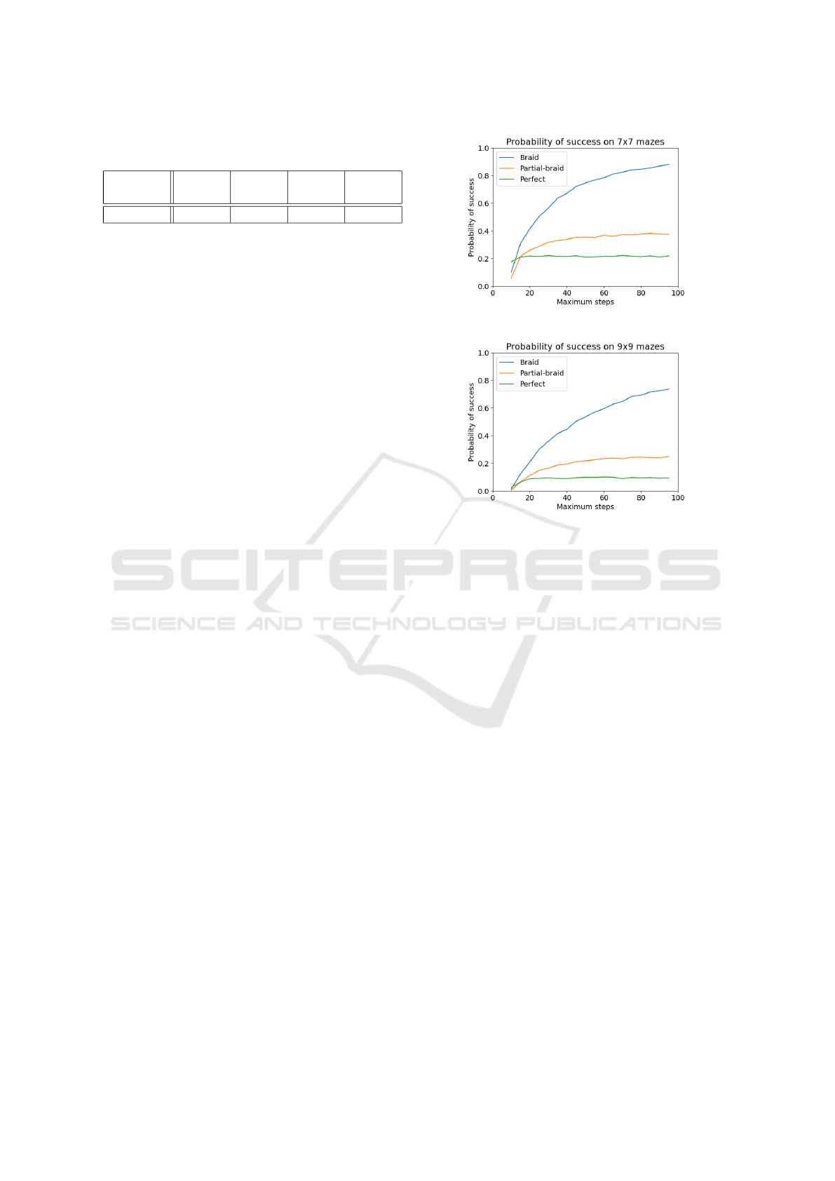
Table 1: HRL baseline successes out of 100 trails on 7x7

mazes.

Test →

Train ↓

Laby-

rinth

Braid Partial

Braid

Perfect

Braid 78 95 96 96

least two openings at each turning section. (See Fig-

ure 1 for examples of this.) The presence of two or

more empty squares allows the agent to execute a

wider turning arc.

The primary purpose of the HRL-baseline was to

demonstrate that with sufﬁcient map information, the

RL approach was capable of overcoming the restric-

tions imposed by Ackermann steering given the tight

conﬁnes of the environments being used.

4.3.2 Random Action Baseline

Given the start and goal locations, the random search

randomly selects adjacent squares which are not

blocked by an obstacle to move to, with the only con-

dition being that it cannot travel to its previous square.

This mimics the behaviour of our Ackermann sim-

ulations, which cannot move backwards. This pre-

vents the random policy from turning into walls “ac-

cidentally”, but the random policy will fail if it enters

a dead end. The random baseline does not enforce

Ackermann constraints on the motion of the vehicle.

The algorithm is run until it reaches the goal square,

crashes at a dead end, or exceeds a maximum number

of steps. Figure 2 shows the probability of success of

the algorithm on a given maze type after a given num-

ber of steps. Each data point was gathered by run-

ning the algorithm on 100 mazes of the given class.

For labyrinth and braid mazes in which there are no

dead ends, the algorithm can only fail by exceeding

the maximum steps, the probability of success will

eventually equal 1. Given the impossibility of failure,

we do not report the random policy’s performance in

Tables 2 or 3.

For both the random baseline and E2E-RL, on per-

fect mazes we assume that the ﬁrst step taken does not

strike a wall. The reference angle of the robot is set in

E2E-RL before we run it, and we select an angle that

gives the agent a chance to reach the goal. Therefore

we give the same beneﬁt to the random search for the

sake of a fair comparison.

4.3.3 E2E-RL

We investigate the performance of E2E-RL on eval-

uation sets of size 100 on 7x7 mazes (Tables 2 and

4), which is the size they were trained on, and on

100 mazes of size 9x9 (Table 3, 5) which represents a

more complex maze than the training set.

(a) 7x7 mazes

(b) 9x9 mazes

Figure 2: Probability of success for random baseline on dif-

ferent maze sizes. Each data point represents running the

algorithm on 100 mazes.

The E2E-RL agents trained on partial-braid and

perfect mazes signiﬁcantly outperform the random

search policy on mazes with dead ends (partial braid

and perfect mazes). Interestingly, the agent trained on

braid mazes did not outperform a random search on

partial-braid mazes. This may be because the lack of

dead ends in braid mazes led the agent to focus on

learning optimal local path execution rather than op-

timal global navigation. This is supported by the fact

that the braid maze agent outperformed all the agents

on the labyrinth mazes, even the labyrinth agent itself.

For both 7x7 and 9x9 mazes the agent trained on

labyrinths performed well on labyrinths and poorly

on the rest. This was expected as this agent had no

need to learn any global navigation behaviour and

could focus solely on local path execution. For 7x7

mazes it is interesting that the agent trained on braid

mazes outperformed the labyrinth agent on its own

maze type. A potential reason for this is that the braid

agent was exposed to more variety in training due to

the numerous paths available given the loops, while

the labyrinth agent was exposed to more simple struc-

tures during training. Perhaps the most striking result

is that the partial braid agent performs very well (the

best or very close to the best) on all classes on the

9x9 maze evaluation. Again, this may be the result of

Nonholonomic Robot Navigation of Mazes using Reinforcement Learning

373

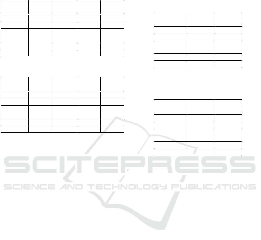
Table 2: E2E-RL successes out of 100 trails on 7x7 mazes.

Best performing policy is in bold.

Test →

Train ↓

Laby-

rinth

Braid Partial

Braid

Perfect

Labyrinth 94 34 23 20

Braid 96 64 35 32

Partial

Braid

83 80 64 49

Perfect 68 78 62 51

Random - - 37 22

Table 3: E2E-RL successes out of 100 trails on 9x9 mazes.

Best performing policy is in bold.

Test →

Train ↓

Laby-

rinth

Braid Partial

Braid

Perfect

Labyrinth 89 29 17 12

Braid 94 52 15 11

Partial

Braid

85 71 46 36

Perfect 53 65 44 34

Random - - 24 9.5

training against more complex environments.

When comparing path lengths for braid and

partial-braid mazes, we selected a maximum number

of steps for the random policy. (Had we not, the ran-

dom policy might never complete when run on braid

or partial braid mazes.) We use a maximum number

of steps cutoff for which the random policy demon-

strated a performance equal to the average perfor-

mance of all the E2E-RL agents over all maze types.

Table 4 reports path length results for 7x7 mazes

and Table 5 reports path length results for 9x9 mazes.

For 7x7 mazes on all classes except labyrinth and

braid, the policy trained on partial braid and perfect

mazes performed best, with the policy trained on per-

fect mazes performing the best on 9x9 mazes over

both braid and partial braid environments. With the

exception of the random policy on the labyrinth and

braid classes, the policy trained on partial braid mazes

was more likely to succeed, especially as 9x9 mazes

were considered, yet the policy trained on perfect

mazes found the path most quickly.

For the labyrinth and braid mazes, the random pol-

icy is guaranteed to ﬁnd a solution if run for a sufﬁ-

ciently long time as the random policy does not set the

turning angle but rather just identiﬁes the next empty

block. As it cannot crash the vehicle, and there are

no dead ends, eventually it will be successful. For

the other policies, the policy does choose the turning

angle and thus even for labyrinth and braid mazes,

failure of the policy is a possible outcome.

Table 4: E2E-RL average path length for successes on 7x7

mazes over 100 trials. 1 unit = width of a cell. Lower

values are better. Best performing policy for each test class

is in bold.

Test →

Train ↓

Braid Partial

Braid

Labyrinth 16.94 11.83

Braid 14.69 13.31

Partial

Braid

11.85 11.00

Perfect 11.95 10.46

Random 19.59 15.85

Table 5: E2E-RL average path length for successes on 9x9

mazes over 100 trials. 1 unit = width of a cell. Lower

values are better. Best performing policy for each test class

is in bold.

Test →

Train ↓

Braid Partial

Braid

Labyrinth 22.69 16.70

Braid 22.27 20.00

Partial

Braid

16.39 14.17

Perfect 15.14 13.63

Random 27.08 22.98

4.4 Real World Validation

The simulations used above make strong assumptions

about the ability of a robot to obtain good odometry

and orientation information, and to be able to capture

and use simulated LIDAR to obtain state information

about obstacles in the environment. In order to vali-

date these assumptions we conducted indoor and out-

door experiments with a wheeled mobile robot. These

experiments did not validate end to end performance

of the policies developed here, but rather were used

to validate the ability of obtaining state information

and providing action information to a real robot. For

real world experiments, a E2E-RL navigation func-

tion trained on braid mazes.

Experiments were performed using an Adept skid-

steer P3-AT base augmented with LIDAR, GPS re-

ceiver, gyroscope and on board computation. The

P3-AT’s skid steer was used to simulate Ackermann

kinematics. Given the size of the P3-AT, for real

world validation the cell size in the maze was set to

2.2m x 2.2m. Space did not permit testing on full

7x7 mazes, as such mazes would require 15m x 15m

testing environments and the construction of hundred

of meters of temporary walls, so real world experi-

ments were limited to smaller maze structures to ex-

plore the ability of the E2E-RL algorithm to navigate

complex junctions and corners in the maze. Custom

ICINCO 2022 - 19th International Conference on Informatics in Control, Automation and Robotics

374

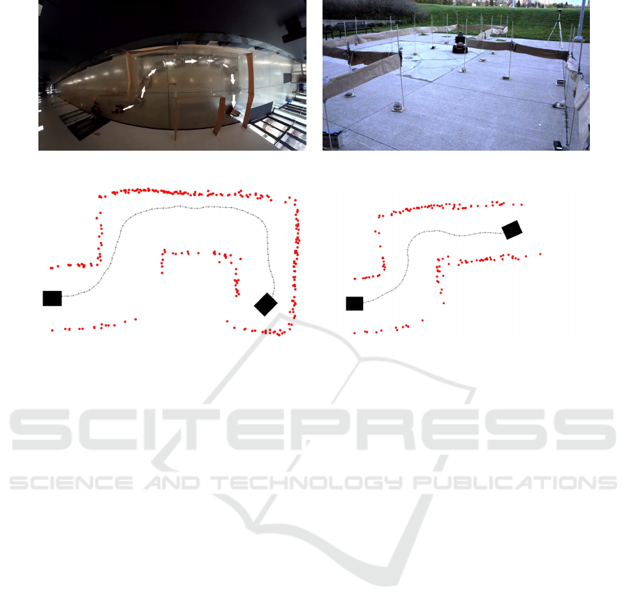
(a) Indoor environment (b) Outdoor environment

Figure 3: Real world navigation. Indoor and outdoor environments and snapshots of the motion of the robot as recorded by

ROS.

ROS nodes were developed to control the robot from

an off-robot control station. Uncertain weather condi-

tions required that experiments be conducted both in-

doors and out. For localization outdoors, a Real-Time

Kinematic (RTK) Global Positioning System (GPS)

(NovAtel, 2020) was used. For indoor localization,

where GPS signals were not available, hand measure-

ments were used as a replacement for the GPS mea-

surement. Although there are more precise automated

methods for indoor localization such as WiFi localiza-

tion (Sun et al., 2014), hand measurement was used

here. For orientation information a gyroscope (Pas-

saro et al., 2017) was used to determine orientation

and angular velocity. A Phidget Spatial sensor (Phid-

gets, 2020) was mounted on the robot and data pro-

vided to the ROS stack. For obstacle detection, the

YDLidar G4 was used. This LIDAR provides denser

samples than the nine used in the policies developed

here, but the signal was sampled to obtain the nine-

dimensional range signal.

4.4.1 Indoor Experiments

Indoor experiments were conducted in the Sher-

man Health Sciences Building at York University in

Toronto, Canada. In order to construct a sufﬁciently

complex environment of the correct scale, existing

walls in the building were supplemented with mov-

able wall obstacles that provided a wall like barrier

that could be captured by the LIDAR (Figure 3(a)).

Given the complexity of estimating vehicle position,

indoor experiments were quite time consuming, but

these demonstrated that the assumptions that under-

lie the DRL navigation algorithm applied in this envi-

ronment. The navigation function was successful for

100% on the three indoor environments constructed.

Each test required approximately 12m of robot mo-

tion through the maze. Figure 3(c) shows the success-

ful navigation of part of an indoor maze.

4.4.2 Outdoor Validation

Outdoor experiments were conducted on the con-

crete/stone apron adjacent to the Sherman Health Sci-

ences Building at York University (Figure 3(b)). This

apron was sufﬁciently large to permit a range of dif-

ferent junctions to be modelled and navigated. Four

test environments were constructed and the naviga-

tion function was successful in navigating all of them.

The paper “LIDAR walls” used to construct the en-

vironment were impacted by the windy conditions

present during the experiments, and the uneven con-

crete apron around the building impacted vehicle mo-

tion and LIDAR angle relative to the ground plane.

Although this produced a much more noisy LIDAR

signal (visible in Figure 3(d)) and introduced noise

into the motion executed by the vehicle, for the four

outdoor tests the robot was successful in making its

Nonholonomic Robot Navigation of Mazes using Reinforcement Learning

375

way to the goal location. Each test required approxi-

mately 15m of robot motion through the maze.

5 SUMMARY AND FUTURE

WORK

Evaluation of end-to-end RL on different environment

types with non-holonomic vehicles showed the ad-

vantage of training on more complex environments

(partial braid and perfect mazes) in terms of both

probability of success and the length of the found path

to the goal. Validation with real hardware demon-

strated that the assumptions made in terms of the E2E-

RL formulation were realistic.

ACKNOWLEDGEMENTS

This work was supported by the Natural Sciences and

Engineering Research Council (NSERC) through the

NSERC Canadian Robotics Network (NCRN).

REFERENCES

Devo, A., Costante, G., and Valigi, P. (2020). Deep

reinforcement learning for instruciotn following vi-

sual navigation in 3d maze-link environments. IEEE

Robotics and Autonomation Letters, January.

Dudek, G. and Jenkin, M. (2000). Computational Princi-

ples of Mobile Robotics. Cambridge University Press,

Cambridge, UK.

Faust, A., Ramirez, O., Fiser, M., Oslund, K., Francis,

A., Davidson, J., and Tapia, L. (2018). PRM-RL:

Long-range robotic navigation tasks by combining re-

inforcement learning and sampling-based planning. In

IEEE International Conference on Robotics and Au-

tomation (ICRA), Brisbane, Australia.

Haarnoja, T., Zhou, A., Abbeel, P., and Levine, S. (2018).

Soft actor-critic: Off-policy maximum entropy deep

reinforcement learning with a stochastic actor. Inter-

national Conference on Machine Learning (ICML).

Hill, A., Rafﬁn, A., Ernestus, M., Gleave, A., A, K.,

Traore, R., Dhariwal, P., Hesse, C., Klimov, O.,

Nichol, A., Plappert, M., Radford, A., Schulman,

J., Sidor, S., and Wu, Y. (2018). Stable Baselines.

https://github.com/hill-a/stable-baselines.

Karaman, S. and Frazzoli, E. (2011). Sampling-based algo-

rithms for optimal motion planning. The International

Journal of Robotics Research, 30:846–894.

Lavalle, S. M. (1998). Rapidly-exploring random trees: A

new tool for path planning. Computer Science Depart-

ment, Iowa State University.

Matthews, W. H. (1927). Mazes and Labyrinths: Their

History and Development. Dover. Dover Publication

Reprint, 1970.

Mnih, V., Badia, A. P., Mirza, M., Graves, A., Lillicrap,

T. P., Harley, T., Silver, D., and Kavukcuoglu, K.

(2016). Asynchronous Methods for Deep Reinforce-

ment Learning. International Conference on Machine

Learning (ICML).

Mnih, V., Kavukcuoglu, K., Silver, D., Graves, A.,

Antonoglou, I., Wierstra, D., and Riedmiller, M.

(2013). Playing Atari with deep reinforcement learn-

ing. CoRR.

NovAtel (2020). Real-time kinematic (rtk).

https://novatel.com/an-introduction-to-gnss/chapter-

5-resolving-errors/real-time-kinematic-rtk. Accessed:

2020-07-30.

Passaro, V. M. . N., Cuccovillo, A., Vaiani, L., Carlo, M.,

and Campanella, C. E. (2017). Gyroscope technology

and applications: A review in the industrial perspec-

tive. Sensors, 17(10):2284.

Phidgets (2020). Phidgets spatial user guide.

https://www.phidgets.com/. (accessed August

12, 2020).

Pullen, W. D. (2020). Maze classiﬁcation.

https://www.astrolog.org/labyrnth/algrithm.htm.

(accessed August 12, 2020).

Schulman, J., Moritz, P., Levine, S., Jordan, M., and

Abbeel, P. (2015). High-dimensional continuous con-

trol using generalized advantage estimation. CoRR.

Silver, D., Huang, A., Maddison., C., Guez, A., Sifre, L.,

van den Driessche, G., Schrittwieser, J., Antonoglou,

I., Panneershelvam, V., Lanctot, M., Dieleman, S.,

Grewe, D., Nham, J., Kalchbrenner, N., Sutskever, I.,

Lillicrap, T., Leach, M., Kavukcuoglu, K., Graepel,

T., and Hassabis, D. (2016). Mastering the game of

Go with deep neural networks and tree search. Na-

ture, 529(7587):484–489.

Sun, Y., Liu, M., and Meng, M. Q. (2014). Wiﬁ signal

strength-based robot indoor localization. In IEEE In-

ternational Conference on Information and Automa-

tion (ICIA), pages 250–256, Hailar, China.

Tai, L., Paolo, G., and Liu, M. (2017). Virtual-to-real deep

reinforcement learning: Continuous control of mobile

robots for mapless navigation. In IEEE/RSJ Interna-

tional Conference on Intelligent Robots and Systems

(IROS), Vancouver, Canada.

Turidus (2017). Python-Maze.

https://github.com/Turidus/Python-Maze.

Wanmg, J., Elfwing, S., and Uchibe, E. (2021). Modular

deep reinforcement learning from reward and punish-

ment for robot navigation. Neural Networks, 135:115–

126.

ICINCO 2022 - 19th International Conference on Informatics in Control, Automation and Robotics

376