Machine Learning Techniques for Breast Cancer Detection

Karl Hall

, Victor Chang

and Paul Mitchell

School of Computing, Engineering and Digital Technologies, Teesside University, Middlesbrough, U.K.

Department of Operations and Information Management, Aston Business School, Aston University, Birmingham, U.K.

Keywords: Cancer Diagnosis, Machine Learning, Support Vector Machine, Algorithm Tuning.

Abstract: Breast cancer is the second most prevalent type of cancer overall and the most frequently occurring cancer in

women. The most effective way to improve breast cancer survival rates still lies in the early detection of the

disease. An increasingly popular and effective way of doing this is by using machine learning to classify and

analyze patient data to help identify signs of cancer. This paper explores a variety of machine learning

techniques and compares their prediction accuracy and other metrics when using the Breast Cancer Wisconsin

(Original) data set using 10-fold cross-validation methods. Of the algorithms tested in this paper, a support

vector machine model using the radial basis function kernel outperformed all other models we tested and those

previously developed by others, achieving an accuracy of 99%.

1 INTRODUCTION

As the prevalence of big data in the healthcare sector

increases (Ehrenstein et al., 2017), there is an

increasing demand for improving the value and

validity of the methodologies employed to help

clinicians make treatment decisions. Traditional,

manual methods to analyze large databases for

meaningful patterns are becoming more difficult as

the size of the databases grows. Instead, we can

analyze these larger data repositories with technology,

including machine learning techniques and statistical

analysis.

Cancer is a collection of deadly diseases and

involves the uncontrollable growth and reproduction

of cells in a specific organ of the body, developing

into a tumor. Breast cancer makes up roughly 25% of

all cancers in women (Clinton et al., 2020) and is the

most common type of cancer in women altogether. In

2020, there were 2.3 million cases and 685,000 deaths

worldwide (World Health Organization, 2021).

In breast cancer, this mostly occurs in the cells

surrounding the breast ducts. Tumors can take two

forms, either malignant or benign. Malignant tumors

can spread to other parts of the body if left untreated.

If a diagnosis of a malignant tumor is given early, the

https://orcid.org/0000-0003-2863-3312

https://orcid.org/0000-0002-8012-5852

* Corresponding authors

chance of a full recovery is significantly higher

(Caplan, May, and Richardson, 2000).

Fine needle aspirate (FNA), ultrasound,

mammography, and surgical biopsies (Mu and Nandi,

2007) are some of the popular techniques currently

used to detect breast cancer. The manual detection of

breast cancer is resource-intensive for physicians and

the difficulty of classification can sometimes be

problematic.

Cancer is one of the most feared diseases, with the

mere thought of it often causing stress and anxiety.

Using technological methods, such as machine

learning, allows healthcare professionals to increase

both the speed of diagnosis and the accuracy of

classification. We aim to contribute to breast cancer

research by improving diagnosis times through the

optimization of machine learning algorithms to

improve the success rate of breast cancer treatment.

This was achieved by fine-tuning the parameters of a

support vector machine (SVM) model using the radial

basis function (RBF) kernel, giving better results than

previous work in this domain.

116

Hall, K., Chang, V. and Mitchell, P.

Machine Learning Techniques for Breast Cancer Detection.

DOI: 10.5220/0011123200003197

In Proceedings of the 7th International Conference on Complexity, Future Information Systems and Risk (COMPLEXIS 2022), pages 116-122

ISBN: 978-989-758-565-4; ISSN: 2184-5034

2 RELATED WORKS

Several studies have been carried out to improve

current analysis methods and study breast cancer

survival in general. Many different approaches have

been taken, which have resulted in a high

classification accuracy.

The mathematical method of multi-surface pattern

separation that was applied to the diagnosis of breast

cytology was initially proposed over 30 years ago

(Wolberg and Mangasarian, 1990). They found the

correct separation in 369 out of 370 samples. These

groundbreaking techniques are still used today.

Decision table models have been used to predict

the survival rates of breast cancer (Liu et al., 2009).

They found that the survival rate was 86.5%. They

used C5 node techniques and bagging algorithms to

improve predictive performance.

Logistic regression models, artificial neural

networks, and C5 node decision trees have also been

used (Delen et al., 2005) using 10-fold cross-

validation methods to predict the survival outcome of

over 200,000 breast cancer patients. They found that

their C5 node decision tree gave the highest

predictive accuracy at 93.6% out of the models used.

Investigations of a variety of medical data sets to

determine whether the performance of K-nearest

neighbor (KNN) models is affected by the distance

function have been conducted (Hu et al., 2016). They

looked at different types of data, including mixed,

categorical, and numerical data. They also explored

different types of distance functions, such as

Minkowski, Cosine, Euclidean and Chi-Square. They

concluded that the best type of distance function to

use were Chi-Square functions.

Comparisons of the accuracy of various

supervised learning models, including RBF neural

networks, Decision Trees implementing the Iterative

Dichotomiser 3 (ID3) algorithm, Naïve Bayes and

SVM- RBF kernel, were conducted (Chaurasia and

Pal, 2014a) to determine which models are the most

useful at classifying breast cancer datasets. The most

accurate model they tested was an SVM model using

a radial basis function kernel (SVM-RBF) which

achieved a score of 96.8%.

In another study, they also explored the use of data

mining algorithms and their effectiveness at

diagnosing heart disease (Chaurasia and Pal, 2014b).

They concluded that the Classification and Regression

Trees (CART) algorithm gave the highest accuracy.

The effectiveness of SVM, KNN and probabilistic

neural networks at detecting breast cancer was

explored (Osareh and Shadgar, 2010). They combined

this with rankings of signal-to-noise ratio features and

other techniques. The highest accuracy they achieved

was 98.80% by using an SVM-RBF classifier.

A study to compare the effectiveness of Bayesian

models, KNN, SVM, Multilayer Perceptron (MP),

Random Forest (RF) and Logistical Regression (LR)

was conducted using the same Breast Cancer

Wisconsin (Original) data used in this paper (Erkal

and Ayyildiz, 2021). They found their Bayesian

Network performed the best, returning an accuracy of

97.1%.

3 DATASET

The machine learning algorithms demonstrated in this

paper were trained and tested using the Breast Cancer

Wisconsin (Original) data set. The information was

obtained by digitizing images of the FNA of a breast

mass. This data set can be used to predict whether the

cancer cells among numerous patients are benign or

malignant. The data set is made up of nine attributes

of the cell nucleus, along with a benign or malignant

cancer type classification:

•

Clump thickness 1-10

•

Uniformity of cell size: 1-10

•

Uniformity of cell shape: 1-10

•

Marginal adhesion: 1-10

•

Single epithelial cell size: 1-10

•

Bare nuclei: 1-10

•

Bland chromatin: 1-10

•

Normal nucleoli: 1-10

•

Mitoses: 1-10

•

Predicted class: 2 for benign, 4 for malignant

In the digitized images of the breast tissue,

malignant tumor images show the cell nuclei to be

inconsistently sized and asymmetrical. Conversely,

benign tumor cells are usually uniform in their shape

and size. This can be seen in Figure 1, with benign

cells on the left next to the malignant cells on the

right.

Figure 1: Medical image of benign and malignant cancer

cells. (Sizilio et al., 2012).

Machine Learning Techniques for Breast Cancer Detection

117

4 METHODOLOGY

This paper uses three types of supervised learning

classifiers: various kernels of Support Vector Machine,

K-nearest Neighbor and an Artificial Neural

Network. The SVM and KNN models were implemented

using the “Sklearn” library in Python, while the ANN

model was implemented using the “neuralnet” package in

R. Supervised learning models were chosen because

the data set contains information about the cancer

cells, allowing this information to be used as inputs

and corresponding outputs. Supervised models

perform particularly well when they are given

classification tasks with labeled data.

Data cleaning was undertaken before the

implementation of any algorithms. Incomplete or

duplicate entries were removed from the data set and

other checks to ensure the data was consistent. For

example, users should ensure that all data for each

attribute fell within the valid ranges (1-10).

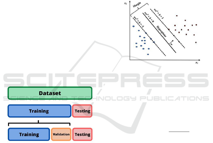
The data was split into segments for training,

testing and validation. Analytics for each model were

obtained, including accuracy, precision, and recall

scores to compare the effectiveness of the models.

The ratio of training data to testing data used was

80:20. A visualization of this process can be seen in

Figure 2.

Figure 2: Visualization of data partition segments.

4.1 Support Vector Machine

SVMs possess the capability of processing multiple

and continuous categorical variables. The SVM

constructs a hyperplane that corresponds to the

training data. The testing data is then classified

alongside the training data on this hyperplane. The

maximum marginal hyperplane is then calculated.

The margin of an SVM is defined as the distance

between the two nearest support vectors relating to the

different classes. In this case, the class refers to benign

and malignant cancer classifications. The larger the

margin, the stronger the classification. A visualization

of this process can be seen in Figure 3. The SVM

algorithm employs cross-fold validation techniques.

The optimal value for this was determined to be 10,

which results in estimates with moderate variance and

low bias (Chaves et al., 2009). In summary, this

process was repeated ten times to improve

consistency. There are different kernels that can be

used in SVM classifiers, such as RBF and polynomial,

with linear being the default kernel. In this case,

kernels define the functions that define the decision

boundaries between classes. These kernels were

compared to optimize the SVM model further.

Figure 3: SVM hyperplane and margins (Huang et al.,

2018).

4.1.1 Radial Basis Function Kernel

In contrast to the linear kernel, the RBF kernel is a

non-linear kernel often used when class boundaries

are hypothesized to be curve-shaped. By given two

samples x and x’, as feature vectors, the RBF kernel

is defined as:

𝐾

(

𝑥,𝑥



)

𝑒𝑥𝑝

𝑥𝑥





2𝜎





(1)

where |

𝑥𝑥





is defined as the squared Euclidian

distance between the feature vectors (Vert, Tsuda and

Schölkopf, 2004). The performance of the RBF

kernel is primarily affected by the adjustment of the

parameter 𝜎 and the cost value.

4.1.2 Polynomial Kernel

The polynomial kernel, more commonly known as

SVM-Poly, is another non-linear kernel representing

the similarity of vectors in the feature space over

polynomials of the original variables. For

polynomials of degree d, the kernel can be defined as:

𝐾

(

𝑥,𝑦

)

(𝑥𝑇𝑦+𝑐)



(2)

COMPLEXIS 2022 - 7th International Conference on Complexity, Future Information Systems and Risk

118

where x and y are vectors of features from testing and

training samples and c is the cost value.

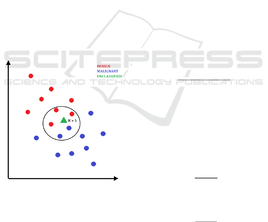
4.2 K-nearest Neighbor

Instead of using training data like most supervised

algorithms, the lazy learning of KNN updates in real-

time as new data points are added. When this occurs,

the classification of k pre-existing data points is

considered to determine the new data classification

depending on proximity. The k-value is the number of

nearby data points considered for this classification.

This process is visualized in Figure 4. In this case, the

new data point visualized as a green triangle would be

classified as benign.

The square root of the number of observations was

calculated to determine the optimal k-value for our

data set. This gives a value of 21.8. Therefore,

initially, two KNN models with k-values of 21 and 22

were running.

Aiming to ensure that 21 and 22 were the best k-

values, the accuracy percentage was calculated for

both, and confusion matrices were produced. A loop

was then created to run this process for all values

between 1 and 28. Finally, a graph was plotted to find

any correlation between the k-values and the accuracy

percentages.

Figure 4: Classification of a new data point with KNN.

4.3 Artificial Neural Network

The ANN uses the seed setting function to produce a

sample for the training segments. The independent

variable x was used as the starting point for the input

layer vector.

Two hidden layers were used for the network, with

each consisting of six neurons. The output layer

consists of the dependent variable y, corresponding to

the cancer class. The output layer outputs either

malignant or benign as response variables. Each value

of x was used to calculate the most likely value of y.

This was calculated by using regression algorithms

that output the corresponding values of y based on a

finite number of noisy x measurements

(Gholamrezaei and Ghorbanian, 2007).

The measurements for the nine independent

variables are obtained by the ANN as weights as they

pass through the ANN from the input layer towards

the output layer. A bias, b, is added to the neurons and

the weight values are modified as the data travels

through the hidden layers. This bias forms the net

input, n, by summing with the weighted inputs using

an activation function (Demuth and Beale, 2000).

This sum is defined as the argument of the transfer

function f (Landis and Koch, 1977).

5 RESULTS AND DISCUSSION

For each of the models, three main metrics were

obtained to assess their performance. The accuracy

score quantifies the percentage of predictions the

classifier got right and is defined in (3).

𝑇𝑃+𝑇𝑁

𝑇𝑃+𝑇𝑁+𝐹𝑃+𝐹𝑁

(3)

where TP = true positive, TN = true negative, FP =

false positive and FN = false negative. A true positive

refers to when the model correctly classifies a positive

result, a true negative is when the model correctly

classifies a negative result, a false positive is when a

positive result is incorrectly predicted, and a false

negative is when a negative result is incorrectly

predicted,

Recall, or sensitivity measures the number of

correct positive predictions made from all possible

positive predictions and is defined in (4).

𝑇𝑃

𝑇𝑃+𝐹𝑁

(4)

The F1 score combines precision (P) and recall

(R), considering both false positives and negatives and

is defined in (5).

2(𝑃∗𝑅)

𝑃+𝑅

(5)

Machine Learning Techniques for Breast Cancer Detection

119

5.1 Support Vector Machine

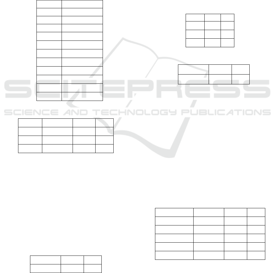
The c-value, or cost value to be used, was determined

using linear grids. The SVM was trialed using

different c-values ranging from 0.01 to 2.5. The best

c-value was shown to be 0.05 (Table 1). By using this

c-value, linear, RBF and polynomial kernels were

tested to compare their accuracy, recall and F1 scores.

A comparison of results is shown in Table 2. From

these results, it can be concluded that SVM-RBF

performs the best compared to SVM-Linear and

SVM-Poly.

Table 1: Comparison of SVM c-values.

c-value

Accuracy (%)

0.01

96.67

0.05

97.22

0.10

96.94

0.25 97.01

0.50 97.01

0.75 97.01

1.00 96.94

1.25 96.94

1.50 96.87

1.75 96.87

2.00 96.94

Table 2: Comparison of SVM kernels.

Kernel Accuracy Recall F1

Linear 97.3 97.8 97.5

RBF 99.0 97.8 98.3

Poly 95.7 94.8 95.2

5.2 K-nearest Neighbor

When the KNN model was tested with the previously

determined optimal k-values of 21 and 22, both

returned an accuracy percentage of 93.55%.

Simulations were run for other k-values to confirm

that 21 and 22 were the optimal k-values. These were

not the optimal values, however. K-values of 3, 6 and

8 all returned higher accuracy percentages of over

94%. Using a k-value of 3 produced the results shown

in Table 3.

Table 3: KNN classifier results.

Accuracy Recall F1

94.5 92.9 93.6

5.3 Artificial Neural Network

The ANN confusion matrix (Table 4) shows the

resulting frequency of the individual data points. The

numbers 2 and 4 correspond to the malignant and

benign classifications, respectively. Of the 123

malignant data points, the network successfully

identified all but one, resulting in 122 true positives

and 1 false negative. Of the 69 benign data points, 66

were true negatives and 3 were false positives.

Overall, the neural network successfully classified

188 out of 192 cancer diagnoses, resulting in an

accuracy score of 97.92%. Table 5 shows the accuracy

along with the other metrics.

Table 4: Neural network confusion matrix.

Ref

Pre

122

Table 5: Neural network classifier results.

Accuracy Recall F1

98.0 96.2 96.7

5.4 Model Comparisons

When looking at all the models in this paper (Table 6),

it can be concluded that the SVM using the RBF

classifier outperformed all the other models across all

metrics used, except for SVM-Linear matching its

recall ability. Furthermore, our SVM- RBF model

outperformed all the models implemented by

previous research, as discussed in Section 2.

Comparisons between our results and those conducted

by other research outlined in Section 2 are shown in

Table 7. The models developed in this paper are

denoted with an asterisk (*) and are shown alongside

models implemented by others.

Table 6: Comparison of all models.

Models

Accuracy Recall

SVM-RBF

99.0 97.8 98.3

ANN

98.0 96.2 96.7

SVM-Linea

97.3 97.8

97.5

SVM-Pol

95.7 94.8 95.2

KNN

94.5 92.9 93.6

COMPLEXIS 2022 - 7th International Conference on Complexity, Future Information Systems and Risk

120

Table 7: Comparison of our models to past research.

Models

Accuracy Recall

SVM-RBF*

99.0 97.8 98.3

SVM-RBF

(Osareh and Shadgar,

2010)

98.8 N/A N/A

ANN*

98.0 96.2 96.7

SVM-Linear*

97.3 97.8

97.5

SVM-RBF (Chaurasia

and Pal, 2014)

96.8 N/A N/A

SVM-Pol

95.7 94.8

95.2

KNN*

94.5 92.9 93.6

DT-C5

(Delen, Walker and

Kadam, 2005)

93.6 N/A N/A

6 ETHICS

We have demonstrated a high level of ethics as

follows. First, all the data has been kept anonymous.

We do not reveal any patients’ identities. Second, the

work we do is fully GDPR compliant. We are only

allowed to analyze data that we have the permission

to use, which does not enclose any sensitive data at

all. Third, our results and analyses do not reveal any

patient identities or any sensitive information. Fourth,

we follow strict privacy regulations and data

governance to ensure the integrity and ethics of our

work. We retain a high level of professionalism and

responsibility towards the ethical use of the data and

the ethical requirements in performing data

processing, analysis and visualization.

Our research follows an ethical framework for

breast cancer detection. In other words, we design,

deploy and validate our algorithms that follow ethical

requirements. Our analyses do not reveal or leak any

sensitive information. Any scientific work, including

machine learning algorithm and development, are

only used on top of following ethical requirements

and compliance.

7 CONCLUSION

With the increasing popularity of big data in the

healthcare sector, larger data sets are becoming

available. One concern throughout this project was

the size of the data set used. The Breast Cancer

Wisconsin (Original) data set consists of less than 700

entries. Different machine learning algorithms

perform better or worse depending on the size of the

data set and the number of data features that can

impact the outcome. SVM algorithms traditionally

perform very well at binary classification problems

with pre-labeled data, which can explain why SVM-

based models outperform other models when using this

data set, in both this paper and work conducted by

others.

Other machine learning techniques for

classification problems could prove even more

accurate than those explored in this paper when

implemented with a more modern approach. Neural

networks and other deep learning algorithms tend to

perform well on very large data sets. When given a

larger and more complex data set, it can be

hypothesized that neural networks would see an

increase in performance compared to other models.

Therefore, one suggestion for future direction in this

area is to explore how different sizes of data sets impact

on the performance of machine learning algorithms.

Random Forest, XGBoost, LightGMB and

CatBoost are examples of increasingly popular

algorithms that can be utilized for handling

classification problems as part of future research to

aid early disease diagnosis. These algorithms fall

under the category of ensemble learning algorithms,

whereby multiple models are integrated

simultaneously and often achieve better performance

than singular models. Additionally, our work is fully

ethical and GDPR compliant and follows strict

privacy and data protection.

It is also possible that a similar approach of

adapting and improving machine learning models for

uses on binary-class data sets can be utilized to

improve medical outcomes for other diseases in the

future, such as COVID-19 and diabetes.

ACKNOWLEDGEMENTS

The Breast Cancer Wisconsin (Original) data set used

in this paper was obtained from the University of

Wisconsin Hospitals, Madison, from Dr. William H.

Wolberg. This work is partly supported by VC

Research (VCR 0000174) for Prof. Chang.

REFERENCES

Caplan, L. S., May, D. S., & Richardson, L. C. (2000). Time

to diagnosis and treatment of breast cancer: results from

the National Breast and Cervical Cancer Early

Detection Program, 1991-1995. American journal of

public health, 90(1), 130.

Machine Learning Techniques for Breast Cancer Detection

121

Chaurasia, V., & Pal, S. (2014a). Data mining techniques:

to predict and resolve breast cancer survivability.

International Journal of Computer Science and Mobile

Computing IJCSMC, 3(1), 10-22.

Chaurasia, V. and Pal, S. (2014b). Performance analysis of

data mining algorithms for diagnosis and prediction of

heart and breast cancer disease. Review of research,

3(8).

Chaves,

R.,

Ram´ırez,

J.,

Go´rriz,

J.,

Lo´pez,

M.,

Salas-Gonzalez, D., Alvarez, I., and Segovia, F. (2009).

Svm-based computer-aided diagnosis of the

Alzheimer’s disease using t-test nmse feature selection

with feature correlation weighting. Neuroscience

let- ters, 461(3):293–297.

Clinton, S. K., Giovannucci, E. L., and Hursting, S. D.

(2020). The world cancer research fund/american

institute for cancer research third expert report on diet,

nutrition, physical activity, and cancer: impact and

future directions. The Journal of nutrition, 150(4):663–

671.

Delen, D., Walker, G., and Kadam, A. (2005). Predicting

breast cancer survivability: a comparison of three data

mining methods. Artificial intelligence in medicine,

34(2):113–127.

Demuth, H. and Beale, M. (2000). Neural network toolbox

user’s guide.

Ehrenstein, V., Nielsen, H., Pedersen, A. B., Johnsen, S. P.,

and Pedersen, L. (2017). Clinical epidemiology in the

era of big data: new opportunities, familiar challenges.

Clinical epidemiology, 9:245.

Erkal, B., & Ayyıldız, T. E. (2021, November). Using

Machine Learning Methods in Early Diagnosis of

Breast Cancer. In 2021 Medical Technologies Congress

(TIPTEKNO) (pp. 1-3). IEEE.

Gholamrezaei, M. and Ghorbanian, K. (2007). Rotated

general regression neural network. In 2007

International Joint Conference on Neural Networks,

pages 1959– 1964. IEEE.

Hu, L.-Y., Huang, M.-W., Ke, S.-W., and Tsai, C.F. (2016).

The distance function effect on k-nearest neighbor

classification for medical datasets. Springer Plus,

5(1):1–9.

Huang, S., Cai, N., Pacheco, P. P., Narrandes, S., Wang, Y.,

and Xu, W. (2018). Applications of support vector

machine (svm) learning in cancer genomics. Cancer

genomics & proteomics, 15(1):41–51.

Landis, J. R. and Koch, G. G. (1977). The measurement of

observer agreement for categorical data. Biometrics,

pages 159–174.

Liu, Y.-Q., Wang, C., and Zhang, L. (2009). Decision tree

based predictive models for breast cancer survivability

on imbalanced data. In 2009 3rd international

conference on bioinformatics and biomedical

engineering, pages 1–4. IEEE.

Mu, T. and Nandi, A. K. (2007). Breast cancer detection

from fna using svm with different parameter tuning

systems and som–rbf classifier. Journal of the Franklin

Institute, 344(3-4):285–311.

Osareh, A. and Shadgar, B. (2010). Machine learning

techniques to diagnose breast cancer. In 2010 5th

international symposium on health informatics and

bioinformatics, pages 114–120. IEEE.

Sizilio, G. R., Leite, C. R., Guerreiro, A. M., and Neto, A.

D. D. (2012). Fuzzy method for pre-diagnosis of breast

cancer from the fine needle aspirate analysis.

Biomedical engineering online, 11(1):1–21.

Vert, J. P., Tsuda, K., & Schölkopf, B. (2004). A primer on

kernel methods. Kernel methods in computational

biology, 47, 35-70.

WHO (2021, Mar. 26). Breast cancer [Online]. Available:

https://www.who.int/news-room/fact-

sheets/detail/breast-cancer

Wolberg, W. H. and Mangasarian, O. L. (1990). Multi-

surface method of pattern separation for medical

diagnosis applied to breast cytology. Proceedings of the

national academy of sciences, 87(23):9193–9196.

COMPLEXIS 2022 - 7th International Conference on Complexity, Future Information Systems and Risk

122