Principal Component Analysis in Gas Transport Simulation
Anton Baldin
1
, Kl
¨
are Cassirer
1
, Tanja Clees
1,2
, Bernhard Klaassen
1
,
Igor Nikitin
1
, Lialia Nikitina
1
and Sabine Pott
1
1
Fraunhofer Institute for Algorithms and Scientific Computing, Schloss Birlinghoven, 53754 Sankt Augustin, Germany
2
Bonn-Rhine-Sieg University of Applied Sciences, Grantham-Allee 20, 53754 Sankt Augustin, Germany
Anton.Baldin, Klaere.Cassirer, Tanja.Clees, Bernhard.Klaassen, Igor.Nikitin, Lialia.Nikitina,
Keywords:
Complex Systems Modeling and Simulation, Non-linear Systems, Applications in Energy Transport.
Abstract:
In this paper, an analysis of the error ellipsoid in the space of solutions of stationary gas transport problems
is carried out. For this purpose, a Principal Component Analysis of the solution set has been performed. The
presence of unstable directions is shown associated with the marginal fulfillment of the resistivity conditions
for the equations of compressors and other control elements in gas networks. Practically, the instabilities occur
when multiple compressors or regulators try to control pressures or flows in the same part of the network. Such
problems can occur, in particular, when the compressors or regulators reach their working limits. Possible
ways of resolving instabilities are considered.
1 INTRODUCTION
This work continues the study of globally convergent
methods for solving stationary network problems in
the particular case of gas transport networks, which
was initiated in our earlier works (Clees et al., 2018a;
Clees et al., 2018b; Baldin et al., 2020; Baldin et al.,
2021; Clees et al., 2016). In these works, it was
shown that stationary network problems, whose ele-
ments satisfy a generalized resistivity condition, have
a unique solution that can be found by the standard
stabilized Newton method with an arbitrary choice of
starting point. In this paper, we will analyze the errors
in the solution space of the problem using Principal
Component Analysis (PCA).
A globally convergent method for network prob-
lems in the special case of electrical networks was
formulated in (Katzenelson, 1965), its generalizations
for piecewise linear systems were made in (Chien and
Kuh, 1976; Griewank et al., 2015). For smooth sys-
tems, a practical implementation of the globally con-
vergent Newtonian method can be found in (Press
et al., 1992), and the corresponding convergence the-
ory in (Kelley, 1995). More general globally conver-
gent homotopic methods are described in (Allgower
and Georg, 2003).
Modeling of gas transport networks is based on a
number of empirical approximations (Mischner et al.,
2011; Schmidt et al., 2015). For the law of fric-
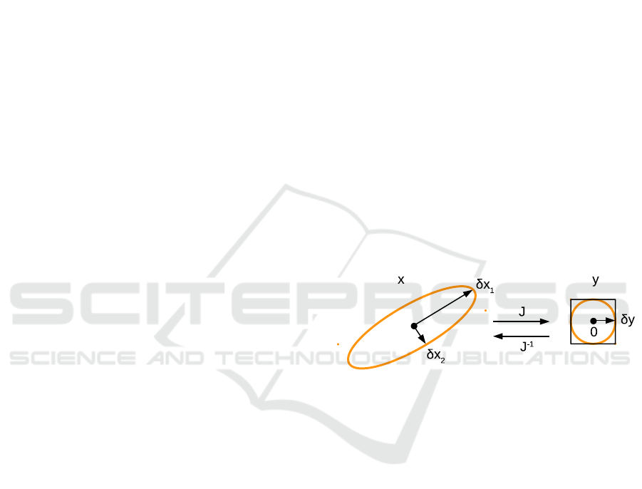
Figure 1: The error ellipsoid in the space of solutions x is
the pre-image of the error ball in the space of equations y
under the linearized mapping J.
tion in pipes, the formulas by Nikuradse, Hofer and
Colebrook-White (Nikuradse, 1950; Colebrook and
White, 1937) are used. For the real gas equation of
state, the formulas by Papay, DIN standard AGA8-
DC92 and improved GERG-2008 (Saleh, 2002; CES,
2010; Kunz and Wagner, 2012) are used. Modeling of
other elements was also described in the works (Clees
et al., 2018a; Clees et al., 2018b; Baldin et al., 2020;
Baldin et al., 2021; Clees et al., 2016) cited above.
This simulation and numerical methods form the ba-
sis of our multi-physics network simulator MYNTS.
First, we will briefly present a problem that occurs
in almost all gas transport applications, since they all
contain elements that increase and decrease pressure,
compressors and regulators correspondingly. If these
elements try to control the pressure at one point, or
in one section of the network, then the correspond-
ing system of equations turns out to be degenerate.
Uncertain values of some variables are a consequence
178
Baldin, A., Cassirer, K., Clees, T., Klaassen, B., Nikitin, I., Nikitina, L. and Pott, S.
Principal Component Analysis in Gas Transport Simulation.
DOI: 10.5220/0011123000003274
In Proceedings of the 12th International Conference on Simulation and Modeling Methodologies, Technologies and Applications (SIMULTECH 2022), pages 178-185
ISBN: 978-989-758-578-4; ISSN: 2184-2841
Copyright
c
 2022 by SCITEPRESS – Science and Technology Publications, Lda. All rights reserved

of this degeneracy; in pressure control, such unsta-
ble variables are flows. To identify such situations
in real problems, we use classical PCA methods. Of
course, these methods are well known and described
in the literature, but the interpretation of their appli-
cation in gas transport problems is very non-trivial
and requires special consideration. Similar methods
have been used in (Chen, 2016) to quantify gas trans-
port in shales. There are also more complex methods
of dimensional reduction available (Hyv
¨
arinen, 2013;
Demartines and Herault, 1997; Lee and Verleysen,
2007).
This paper has the following structure. Section 2
presents the methodology used for the evaluation of
the error of the simulation result in the solution space
of a stationary network problem. In Section 3, the
results of numerical experiments will be presented,
PCA of solutions of a realistic gas transport prob-
lem will be carried out and conclusions will be drawn
about the presence of unstable directions in the solu-
tion space. Section 4 will discuss the obtained insta-
bilities and suggest ways to resolve them.
2 METHODOLOGY
Stationary network simulations belong to a wide class
of problems in which a system of algebraic equations
of the form y(x) = 0, usually large and non-linear, is
solved, where the dimensions of the space of variables
and equations are the same: dimx = dim y = n. Math-
ematically, the solution in x-space is the pre-image
of the point 0 in y-space. The equations are solved
numerically, with a given accuracy |δy| ≤ tol
y
, and
around the point 0 in the y-space, a neighborhood of
admissible solutions arises. This situation is depicted
in Fig.1 on the right. If L
2
-norm is used to estimate
the accuracy, then the neighborhood is spherical, but
if L
∞
-norm is used, that is, max|y|, then the neighbor-
hood is cubic. In the analysis carried out in this paper,
it is more convenient to use the spherical neighbor-
hood and L
2
-norms. To estimate the error in x-space,
the mapping y(x) must be linearized by introducing
the Jacobi matrix J
i j
= ∂y
i
/∂x
j
. The inverse image
of a spherical neighborhood in y-space under a lin-
earized mapping is an ellipsoid in x-space. The values
of the principal semi-axes of the ellipsoid determine
the amplitudes of the δx errors, and their orientation
determines the distribution of the errors over the x-
variables.
Technically, to determine the semi-axes of the
ellipsoid, it is necessary to perform a Singular Value
Decomposition (SVD) of the J matrix:
J = uλv
T
, u
T
u = 1, v
T
v = 1, δx
i
= tol
y
/λ
i
, (1)
where λ is a diagonal matrix, u and v are orthogonal
matrices, δx
i
is the semi-axis corresponding to eigen-
value λ
i
. For nonzero λ
i
, the columns of the v-matrix
determine the position of the semi-axes in the x-space,
the columns of the u-matrix determine the position of
the image of these semi-axes in the y-space. When
λ
i
is zero, the corresponding columns determine the
right and left annulators of the matrix J.
The described procedure is a part of PCA method,
whose purpose is to identify directions in the space
of solutions of the considered problem, which can be
interpreted as the main or most important from the
applied point of view. Such an analysis is easy to
carry out with the help of modern systems of analyti-
cal computations, for example, Mathematica. We will
describe the details of the implementation below, now
we will note some features of the gas transport prob-
lems.
Transport network problems are given by a system
of equations that includes linear Kirchhoff equations
of the form
∑
Q
i
= 0 in each node of the network, de-
scribing the conservation of the flow, and nonlinear
equations of elements of the form f (P
in
,P
out
,Q) = 0
in each edge of the network graph. Here we use the
transport variables P
in/out
assigned to the input and
output nodes, for gas networks – pressures; Q is the
edge-assigned flow. In gas problems, flows are con-
sidered in different normalizations: Q
m
– mass flow,
Q
ν
– molar flow, Q
N
– volumetric flow under normal
conditions, etc. The general formulations do not de-
pend on the type of flow normalization.
It was shown in (Clees et al., 2018a) that if all net-
work elements satisfy the generalized resistivity con-
dition:
∂ f /∂P
in
> 0, ∂ f /∂P
out
< 0, ∂ f /∂Q < 0, (2)
then the Jacobian of the system is nondegenerate and
the problem under consideration has a unique solu-
tion. This solution can be found numerically using
the Newtonian algorithm stabilized by the Armijo line
search rule, with an arbitrary choice of starting point.
Additionally, it is required to have a supply with a
given pressure Pset in each disconnected graph com-
ponent and a proper condition on the behavior of
functions at infinity, which can be satisfied by choos-
ing linear continuations of functions outside the work-
ing region.
The problem faced by practical simulation is the
marginal fulfillment of the rule (2) for some elements.
In particular, the compressor equations are:
Principal Component Analysis in Gas Transport Simulation
179

max(min( P
in
− P
L
,−P
out
+ P
H
,−Q + Q
H
), (3)
P
in
− P
out
,−Q) + ε(P
in
− P
out
− Q) = 0, (4)
with given constants P
L
, P
H
, Q
H
. This equation de-
scribes a polyhedral surface in the space of transport
variables, whose faces P
in
= P
L
, P
out
= P
H
, Q = Q
H
,
etc., are associated with the target values, for exam-
ple, P
H
= SPO , specified output pressure, Q
H
= SM,
specified mass flow, or with technical limits: P
L
=
PIMIN, minimal input pressure, P
in
= P
out
, bypass
mode, Q = 0, OFF mode, etc.
An additional term with a positive small ε serves
as a regularization and was introduced for the follow-
ing reason. Without this term, some derivatives with
respect to transport variables would vanish: for the
face P
in
= P
L
the derivatives with respect to (P
out
,Q)
vanish, for the face P
out
= P
H
– w.r.t. (P
in
,Q), etc.
The geometric interpretation of this property is the di-
rection of the normals to the faces of the polyhedron
along the axes, while the condition (2) requires that
the normals be directed strictly inside the correspond-
ing octant. The presence of such zero derivatives in
certain situations leads to the degeneration of the Ja-
cobi matrix, the disappearance or non-uniqueness of
solutions, and the failure of numerical procedures.
The introduced purely resistive ε-term formally cor-
rects the problem, the condition (2) is satisfied, and
the numerical procedure finds a solution. At the same
time, the ε-term deforms the solution, violates the ex-
act fulfillment of the target equalities P
out
= SPO, etc.
This term must be small enough for the solution to be
physically acceptable. In this case, problems with nu-
merical procedures start to return. The range of values
ε = 10
−6
...10
−3
is acceptable for the most of applica-
tions.
In this paper, in the context of the performed PCA,
we will discuss the following aspect. We will see that
small values of the ε-parameter in certain situations
are associated with eigenvalues close to zero, which
correspond to an almost degenerate Jacobi matrix and
large error values in the space of the problem vari-
ables. Thus, as the solution begins to fulfill the target
equalities more and more accurately, some variables
become less and less precisely defined. This peculiar
uncertainty principle will be discussed in more detail
in Section 4.
The work (Chen, 2016) used the PCA method for
the analysis of gas transport in shales. In general, this
is the same technique that we use to analyze instabil-
ities in the distribution of pressures and flows in gas
networks. In detail, (Chen, 2016) analyzes the depen-
dence of a single curve of pressure decline vs time,
discretized at 5 points, on the variation of a single in-
put parameter, discretized at 100 points, in order to
highlight the main trends in this relationship. In our
case, the PCA is applied to the 200x200 Jacobi ma-
trix in order to detect and classify its degenerate di-
rections.
There are also other factorization techniques, e.g.,
Independent Component Analysis (ICA) (Hyv
¨
arinen,
2013), Curvilinear Component Analysis (CCA) (De-
martines and Herault, 1997), Nonlinear Dimensional-
ity Reduction (Lee and Verleysen, 2007), etc. They
are generalizations of the PCA method for nonlinear
problems, signal processing and other particular ap-
plications, many of them also rely on PCA at their
core. For our purpose of identifying unstable direc-
tions in Jacobi matrix, the basic linear PCA method is
sufficient.
3 RESULTS
We will now apply the PCA algorithm to the gas
network problem N1 depicted in Fig.2. The net-
work has 100 nodes and 111 edges, which include
4 compressors c1-4. The compressors are organized
into two stations c1|2 and c3|4, in each station the
compressors are connected in parallel, as shown in
the lower part of the figure. The station also in-
cludes other elements, but they have trivial equa-
tions and are eliminated by the topological cleaning
filter used in the solution procedure. In this sce-
nario, all compressors are set to P
H
= SPO mode
with the same SPO value. More technical data on
the network used: pipe diameters 0.4-1.2m, pipe
lengths 0.1-57km, incoming pressure Pset=50bar,
compressors setting: SPO=80bar, outcoming flows
Qset(n76) = 300 · 10
3
Nm
3
/h, Qset(n80) = 700 ·
10
3
Nm
3
/h, Qset(n91) = 1000 · 10
3
Nm
3
/h.
As the most important values in this study, the
compressor parameters ε
c12
= 10
−5
, ε
c34
= 10
−6
are
used. The values are deliberately chosen to be differ-
ent to avoid mixing up the corresponding eigenvec-
tors. The simulation is done with the choice tol
y
=
10
−5
. The PCA result is shown in the tables.
Table 1 shows the lowest eigenvalue associated
with ε
c34
. The error in the solution space δx = 513
turns out to be enormously large. Note that the char-
acteristic pressures in the system are on the order of
10-100 bar, the characteristic flows in different nor-
malizations have values of the order of 100-1000, the
equations are also normalized so as to provide an y-
variation of about 100 units in the working region.
Further, the v-column is given in Table 1, the corre-
sponding x-error is localized in station c3|4, and cor-
responds to the disbalance of flows through individual
compressors, when a flow through one compressor is
by δQ larger, through the other – by δQ smaller, and
SIMULTECH 2022 - 12th International Conference on Simulation and Modeling Methodologies, Technologies and Applications
180

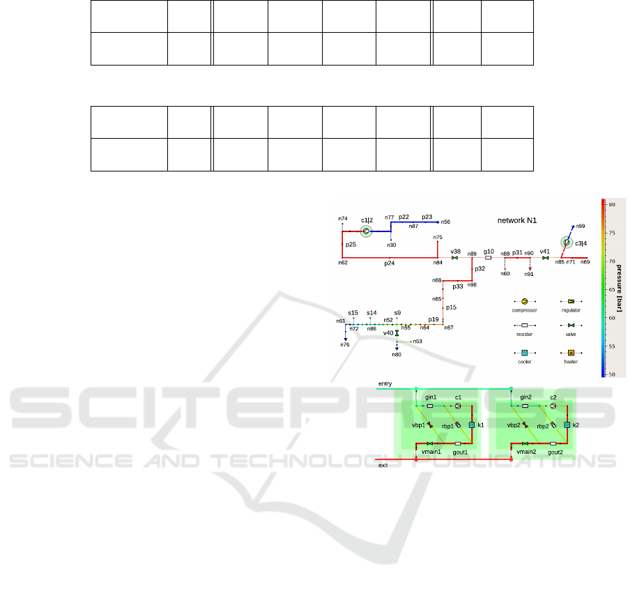
Table 1: The lowest eigenvalue and associated principal components.
λ
1
|δx
1
| δQ
N,c3
δQ
N,c4
δQ
m,c3
δQ
m,c4
eq
c3
eq
c4
1.95 · 10
−8
513 -0.694 0.694 -0.138 0.138 0.707 -0.707
Table 2: The second lowest eigenvalue and associated principal components.
λ
2
|δx
2
| δQ
N,c1
δQ
N,c2
δQ
m,c1
δQ
m,c2
eq
c1
eq
c2
1.95 · 10
−7
51.3 -0.694 0.694 -0.138 0.138 0.707 -0.707
the total flow through the station does not change. In
the problem, flows are introduced in two normaliza-
tions Q
N
and Q
m
, they are also involved in the eigen-
vector with the corresponding coefficients. Next, we
give an u-column that, due to the small eigenvalue,
approximates the left annulator of the matrix J. It is
also localized in the station c3|4 and, in fact, means
that the difference in the control equations is constant.
Indeed, the P
out
= SPO face turns out to be locally ac-
tive in these equations, the equations are identical, and
their difference is zero.
Table 2 shows the second lowest eigenvalue that
happens to be associated with the ε
c12
parameter. In
this case, as expected, the eigenvalue is 10 times
larger, while the error in the solution space δx = 51.3
is 10 times smaller and is still large. The rest of the
table literally repeats the previous one, only the cor-
responding vectors are localized in the station c1|2.
When the ε-parameters change in the range of small
values, eigenvalues change proportionally, while the
eigenvectors do not change.
Table 3 shows the next lowest eigenvalues. Here
the corresponding x-errors turn out to be small. In
addition, the u- and v-vectors are distributed over a
large number of elements, and the error in each ele-
ment is even smaller. The intermediate case is λ
3
=
2.93·10
−4
with the corresponding |δx
3
| = 3.42·10
−2
.
This component is distributed over the pipes connect-
ing the two stations c1|2 and c3|4, suggesting a con-
flict between SPO stations due to the low resistance of
the connecting pipes. This hypothesis is experimen-
tally confirmed, if one artificially increases the length
and/or decreases the diameter of one of the pipes, say,
p24. As a result, the corresponding eigenvalue moves
up and the x-error decreases.
The main result, that ε value has the major influ-
ence to the convergence, has been validated by the
tests on a large network dataset from (Baldin et al.,
2021). It contains 85 real-life networks of complexity
up to 4000 nodes and up to 42 compressors. Setting ε
Figure 2: On the top: test network N1; at the bottom: an
example of parallel compressor station. Images from (Clees
et al., 2018a).
in compressors and regulators to small values leads to
significant degradation of convergence. It should be
emphasized that the ε-singularity is the only problem
for convergence and for slowing down of the solution
process. All other equations were specially processed
(unfolded) by the methods described in (Clees et al.,
2018a; Clees et al., 2018b; Baldin et al., 2020; Baldin
et al., 2021; Clees et al., 2016), in order to ensure sta-
ble non-degeneracy of the Jacobi matrix both inside
and outside the working region. Table 4 gives char-
acteristics of convergence for different values of the
ε-parameter. This test was carried out on one network
N85.1 from the (Baldin et al., 2021) set, which has
∼ 2000 nodes, ∼ 2000 edges, ∼ 200 of which have
potentially singular equations. The timing is given
for a part of the general procedure described in (Clees
et al., 2016), including only the free phase, numeri-
cal solution, without the translation procedure. It can
be seen that for ε ∼ 1 the method requires a moder-
ate number of iterations and is performing fast. How-
Principal Component Analysis in Gas Transport Simulation
181

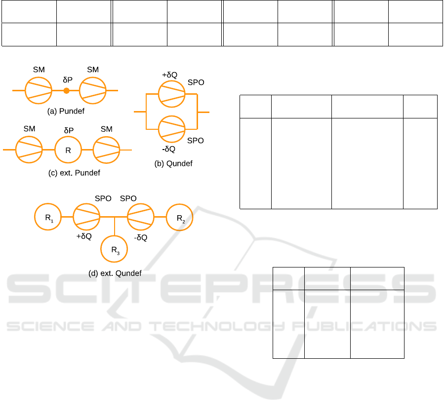
Table 3: The next lowest eigenvalues.
λ
3
|δx
3
| λ
4
|δx
4
| λ
5
|δx
5
| λ
6
|δx
6
|
2.93 · 10
−4
3.42 · 10
−2
3.45 · 10
−2
2.89 · 10
−4
4.79 · 10
−2
2.09 · 10
−4
6.95 · 10
−2
1.44 · 10
−4
Figure 3: Examples of local and extended conflicts in the
formulation of gas transport tasks. See text for the details.
ever, the target values of the obtained solution turn out
to be strongly violated, and the solution is physically
unacceptable. Target values get better as ε decreases,
but the number of Newton iterations and Armijo line
search iterations increases. For the values ε ∼ 10
−6
,
the number of iterations exceeds the established lim-
its, practically meaning the divergence of the method.
Approximately the same trend is shown by other net-
works from the N85 set, with possible statistical out-
liers. Table 5 shows the dependence on ε of the num-
ber of diverged scenarios (out of total 85), as well as
the time to solve all scenarios. Here, timing covers
all phases of the solution, including translation and
initialization; the solution was restricted to free mod-
eling of compressors. These indicators are more sta-
ble to statistical outliers and show an increase in the
number of diverging scenarios and total time, with the
decrease in ε-parameter.
4 DISCUSSION
Problems that may arise in practical scenarios are il-
lustrated in Fig.3. In the ε → 0 limit, a number of
conflicts can occur when compressors are connected
Table 4: Dependence of convergence rate on parameter ε
for network N85.1.
ε Newton iter. line search iter. time*
1 76 404 3
10
−2
152 920 6
10
−4
222 2218 14
10
−6
> 500 23079 div.
* in seconds, for 2.6 GHz Intel i7 CPU 16 GB RAM
computer.
Table 5: Convergence characteristics for all N85 networks.
ε total div. total time*
10
−3
0 8
10
−6
11 15
10
−9
58 53
*in minutes, for 2.6 GHz Intel i7 CPU 16 GB RAM
computer.
in series and in parallel. When compressors are con-
nected in series, with working points located on their
Q
H
-faces, with equal values of Q
H
= SM, after tak-
ing into account the conservation of the flow, each
of the compressors gives the same equation for the
flow: Q = SM. Thus, the equation is repeated twice
and makes the system degenerate. When one equa-
tion is excluded from the system, it turns out to be
underdetermined, that is, the solution has one contin-
uous degree of freedom. A simple check shows that
the pressure in the intermediate node disappears from
the system and is therefore arbitrary. This situation
is depicted in Fig.3a and can be classified as a local
Pundef-conflict.
In the case of parallel connection of compressors
located on their P
out
= P
H
faces, with equal values
of P
H
= SPO, the same equation P
out
= SPO appears
twice in the system. Here, the system also degener-
SIMULTECH 2022 - 12th International Conference on Simulation and Modeling Methodologies, Technologies and Applications
182

ates and a continuous degree of freedom appears in
the solution. This degree of freedom corresponds to
the disbalance of the flows in the compressors, that is,
the addition of ±δQ to the flows canceling each other
in the total flow through the station. In this situation,
shown in Fig.3b, there is a local Qundef-conflict be-
tween the compressors.
The ambiguity is not necessarily limited to the
compressor station, it can also go beyond it. Fig.3c
shows an extended Pundef-conflict. Here two SM-
compressors are connected by an intermediate sub-
graph R, which in a particular case can be a pipeline.
Since there are no equations in the subgraph that
could fix the pressure, it turns out to be undefined
along the pipeline. In a more general case, one can
choose for R any connected subgraph that satisfies
the generalized resistivity conditions and does not in-
clude supplies with a given pressure Pset. Let there
be a solution in which both compressors are stably lo-
cated inside their SM-faces. In this case, they can be
replaced by supplies or exits with given flows Qset.
The solution exists only if these Qsets are balanced
with the Qsets in the subgraph R, that is, their to-
tal sum is zero. Further, by choosing an arbitrary
node of the subgraph R, one can discard the Kirch-
hoff condition written in it, since it follows from the
conservation conditions and is fulfilled automatically.
This condition can be replaced by the P = Pset con-
dition, with the pressure value taken from the chosen
solution. The result of these manipulations is a con-
nected generalized resistive graph with a given Pset,
for which the system has a unique solution. Now Pset
can be shifted by an arbitrary small value δP, and the
solution will also exist and be unique. In this case, by
continuity, the shift of the solution will be arbitrarily
small and still be inside the SM-faces, that is, it will be
a solution to the originally posed problem. As a result,
we have demonstrated the presence of continuous ar-
bitrariness in the solution associated with a change in
pressure, Pundef-conflict. It is also noteworthy that
this consideration can be applied to any node of the R
subgraph, including those with Qset = 0. Therefore,
the arbitrariness affects the pressure at all nodes of the
subgraph.
Similarly, one can get an extended Qundef-
conflict, see Fig.3d. Here, two SPO compressors con-
trol the pressure in one node. The equations repeat,
the system is degenerate, and the solution has a con-
tinuous degree of freedom associated with the ±δQ
disbalance of flows through the compressors. Now
this disbalance extends to the outer subgraphs R
1,2
,
which in a particular case can be pipelines with Psets
at the free ends, and for subgraph R
3
– a pipeline with
Qset at the free end. In a more general case, one can
choose for R
1−3
connected generalized resistive sub-
graphs, for R
1,2
– with Psets, and for R
3
– with Pset or
without it. Next, consider a solution where the com-
pressors are stably inside their SPO-faces. The net-
work can be dissected at compressors into three dis-
connected parts, while for R
1,2
the compressors can
be replaced by Qsets, and for R
3
by Pset = SPO. The
solution exists and is unique in each of these three
subgraphs, while in R
3
the solution does not change
and in R
1,2
it is deformed when ±δQ-flows change.
Thus, we have shown the presence of Qundef-conflict
in the considered scenario.
While the problems of a local type can be noted
and ignored, for extended conflicts, entire network re-
gions may have undefined characteristics, which re-
quires additional analysis. At first glance, the de-
scribed conflicts can be recognized and eliminated,
by an automatic algorithm or manually, for example,
not allowing SPO conditions to collide in the same
node. However, the conflict may arise not between
the main target faces, but between the auxiliary ones,
that is, PIMIN, QMAX and all other conditions in the
equation can enter into conflict. Some of these con-
flicts do not occur directly, but persist through sub-
graphs. It is impossible to predict in advance which
faces will be activated, and consideration of all poten-
tially emerging possibilities for large networks turns
out to be combinatorially unacceptable. Conflict can
also arise at intermediate iterations, on the path from
the starting point to the solution. This will lead to the
degeneration of the Jacobi matrix and to the immedi-
ate divergence of the solution algorithm.
Compressors also have a refined, so-called ad-
vanced model (Clees et al., 2018b; Baldin et al.,
2021) that includes additional conditions in the con-
trol equation. These conditions do not fix the prob-
lem, as they only add new faces that are curved and
with the correct signature, but the old faces still re-
main in the equation and continue to generate con-
flicts. In practice, if the compressor can fulfill its
target conditions, then it is right on those potentially
conflicting faces.
In gas transport problems, not only the compres-
sors bring the described difficulties. Other elements,
in particular, regulators, flaptraps, REPD-resistors,
are also modeled by piecewise linear conditions of
the marginal signature (Clees et al., 2018a). A con-
flict can arise in any combination of these elements,
and also as a result of direct connection of conflicting
faces with Pset or Qset conditions.
It follows from the above formulas that due to the
ε-regularization, the polyhedron faces corresponding
to the control equation are deformed, and the devia-
tions from the target values on the solution turn out to
Principal Component Analysis in Gas Transport Simulation
183

be proportional to ε. At the same time, the errors of
the variables described by the semi-axes of the ellip-
soid are inversely proportional to ε, because of this,
the above mentioned uncertainty principle is fulfilled
– an increase in the accuracy of fulfillment of the
target values for some variables leads to a decrease
in the accuracy of the result for the other variables,
δP · δQ = Const for the Pundef/Qundef-conflicts con-
sidered here.
Theoretically, the slowdown of the solution algo-
rithm with decreasing ε is understandable. Small ε
make the Jacobi matrix almost degenerate, the cor-
responding condition number is large, algorithms for
solving linear systems in Newtonian iterations are less
stable. The size of the Newtonian step dx
N
= −J
−1
y
then becomes very large, h = |dx
N
|  1. Line search
stabilization in this case subdivides the Newtonian
step to reduce the residual |y| while taking many steps
to achieve moderate h = |dx
LS
| ∼ 1. In addition,
the direction of the Newtonian step becomes close
to the right annulator J, which leads to the fact that
along the Newtonian direction for small h the resid-
ual changes little and becomes sensitive to nonlinear
effects. Indeed, the function |y| = c
0
+ c
1
h + c
2
h
2
for
small negative c
1
and moderate positive c
2
has a min-
imum for small positive h = −c
1
/(2c
2
). It forces the
line search algorithm to produce additional subdivi-
sions h  1. In this case, the change in the residual
δ|y| = −c
2
1
/(4c
2
) also turns out to be small, and as
a result, the Newton algorithm is forced to perform
many steps until convergence.
Errors in x-space can be reduced if, in addition to
controlling y-convergence |y| ≤ tol
y
, x-convergence is
controlled: |dx
N
| ≤ tol
x
. Indeed, linearization near
the solution x
0
gives y = Jdx, where dx = x − x
0
,
whence |J
−1
y| = |dx| ≤ tol
x
, the solution in x-space
belongs to the intersection of the error ellipsoid and
the ball of radius tol
x
. Such additional conditions are
sometimes introduced into the stop criterion of the
solution algorithms, but in detail this question is ex-
tremely complicated. In (Kelley, 1995) the stabilized
Newtonian algorithm 8.2.1 nsola does not contain x-
conditions, but namely for it the global convergence
has been proved. In (Press et al., 1992) Chap.9.7,
the newt algorithm contains the x-condition, in the
form of L
∞
-norm of the combined relative and abso-
lute value of the x-step. However, this condition is
imposed with the y-condition not as AND, but as OR,
thus, in the x-space, not the intersection, but the union
of the vicinities is accepted. In this case, situations are
possible when, on the accepted solution, some equa-
tions will not fulfill their y-tolerances. Moreover, the
x-condition in (Press et al., 1992) newt is not imposed
on Newtons |dx
N
|, but on the line search step |dx
LS
|.
As a result, solutions can be accepted with large New-
tonian steps and thus large x-errors. Indeed, we have
already seen that in the case of degenerations large
|dx
N
| and small |dx
LS
| can be obtained. In general, if
the stop criterion is provided with a condition on the
|dx
N
|-step, imposed together with the y-condition as
AND, then in degenerate cases the Newtonian method
will be forced to perform even more iterations, lead-
ing to an additional deterioration in convergence.
From all that has been said, it becomes clear that
the problem under consideration belongs to the ill-
defined class, in the mathematical sense. This does
not mean that it is impossible to solve it, but only
that standard well-tested algorithms do not work for
it, and more sophisticated methods are required. The
ideas for constructing such methods are listed below.
Note that none of them can eliminate the ambiguity in
the solution; this property is determined by the struc-
ture of the considered equations. These methods aim
to find a particular solution in the equivalence class,
avoiding divergences as much as possible and making
a moderate number of iterations.
Methods that can help: relaxed Armijo rule (Kel-
ley, 1995; Baldin et al., 2020); topological reduc-
tion (Baldin et al., 2020); dynamical problem state-
ment; homotopic methods (Allgower and Georg,
2003); solvers for piecewise linear systems (Katzenel-
son, 1965; Chien and Kuh, 1976; Griewank et al.,
2015), also (Allgower and Georg, 2003) Chap.12-15;
pseudo-inverse (Press et al., 1992) Chap.2.6. Con-
sideration of these methods is a topic for our further
work.
5 CONCLUSIONS
In this work, an analysis of the error ellipsoid in the
space of solutions of stationary gas transport prob-
lems was carried out. For this purpose, a Principal
Component Analysis of a solution set was performed,
based on the Singular Value Decomposition of the Ja-
cobi matrix of the corresponding nonlinear system.
On the basis of numerical solution of realistic net-
work examples, as well as theoretically, the presence
of unstable directions is shown associated with the
marginal fulfillment of the resistivity conditions for
the equations of compressors and other control ele-
ments in gas networks. These directions correspond
to conflicts in serial and parallel connections of com-
pressors, leading to uncertain pressure and flow val-
ues in the solutions. Conflicts can also extend beyond
the compressor stations and spread to wide regions of
the network.
SIMULTECH 2022 - 12th International Conference on Simulation and Modeling Methodologies, Technologies and Applications
184

When using ε-regularization of the equations, the
resistivity condition can be enforced and one solution
from the equivalence class can be selected. In this
case, conflicts manifest themselves as ∼ ε deviations
of the controlled variables from the target values and
∼ ε
−1
solution errors in other variables, so that the
deviations satisfy the uncertainty principle of a form
δP · δQ = Const. As ε decreases, the numerical pro-
cedures begin to increase the number of iterations and
finally diverge.
We have briefly listed the algorithms that can help
resolving this problem. Further exploration of these
algorithms is in our future plans.
ACKNOWLEDGMENT
The work has been supported by the project
TransHyDE-Sys, grant 03HY201M.
REFERENCES
Allgower, E. L. and Georg, K. (2003). Introduction to Nu-
merical Continuation Methods. SIAM, Philadelphia.
Baldin, A. et al. (2020). Topological Reduction of Sta-
tionary Network Problems: Example of Gas Trans-
port. International Journal On Advances in Systems
and Measurements, 13:83–93.
Baldin, A. et al. (2021). AdvWarp: A Transformation Al-
gorithm for Advanced Modeling of Gas Compressors
and Drives. In SIMULTECH 2021, pages 231–238.
SCITEPRESS.
CES (2010). DIN EN ISO 12213-2: Natural gas – Calcula-
tion of compression factor. European Committee for
Standardization.
Chen, C. (2016). Multiscale imaging, modeling, and princi-
pal component analysis of gas transport in shale reser-
voirs. Fuel, 182:761–770.
Chien, M. J. and Kuh, E. S. (1976). Solving piecewise-
linear equations for resistive networks. International
Journal of Circuit Theory and Applications, 4:1–24.
Clees, T. et al. (2016). MYNTS: Multi-phYsics NeTwork
Simulator. In SIMULTECH 2016, July 29–31, 2016,
Lisbon, Portugal, pages 179–186. SCITEPRESS.
Clees, T. et al. (2018a). Making Network Solvers Glob-
ally Convergent. Advances in Intelligent Systems and
Computing, 676:140–153.
Clees, T. et al. (2018b). Modeling of Gas Compressors and
Hierarchical Reduction for Globally Convergent Sta-
tionary Network Solvers. International Journal On
Advances in Systems and Measurements, 11:61–71.
Colebrook, C. F. and White, C. M. (1937). Experiments
with Fluid Friction in Roughened Pipes. Mathemati-
cal and Physical Sciences, 161:367–381.
Demartines, P. and Herault, J. (1997). Curvilinear Compo-
nent Analysis: A Self-Organizing Neural Network for
Nonlinear Mapping of Data Sets. IEEE Transactions
on Neural Networks, 8:148–154.
Griewank, A., Bernt, J.-U., Radons, M., and Streubel, T.
(2015). Solving piecewise linear systems in abs-
normal form. Linear Algebra and its Applications,
471:500–530.
Hyv
¨
arinen, A. (2013). Independent component analy-
sis: recent advances. Philosophical Transactions:
Mathematical, Physical and Engineering Sciences,
371:20110534.
Katzenelson, J. (1965). An algorithm for solving nonlin-
ear resistor networks. Bell System Technical Journal,
44:1605–1620.
Kelley, C. T. (1995). Iterative Methods for Linear and Non-
linear Equations. SIAM, Philadelphia.
Kunz, O. and Wagner, W. (2012). The GERG-2008 wide-
range equation of state for natural gases and other
mixtures: An expansion of GERG-2004. J. Chem.
Eng. Data, 57:3032–3091.
Lee, J. A. and Verleysen, M. (2007). Nonlinear Dimension-
ality Reduction. Springer.
Mischner, J. et al. (2011). Systemplanerische Grundla-
gen der Gasversorgung. Oldenbourg Industrieverlag
GmbH.
Nikuradse, J. (1950). Laws of flow in rough pipes. NACA
Technical Memorandum 1292, Washington.
Press, W. H. et al. (1992). Numerical Recipes in C. Cam-
bridge University Press.
Saleh, J. (2002). Fluid Flow Handbook. McGraw-Hill.
Schmidt, M. et al. (2015). High detail stationary optimiza-
tion models for gas networks: model components. Op-
timization and Engineering, 16(1):131–164.
Principal Component Analysis in Gas Transport Simulation
185