DL-CNN: Double Layered Convolutional Neural Networks

Lixin Fu and Rohith Rangineni

Department of Computer Science, University of North Carolina at Greensboro, Greensboro, NC 27401, U.S.A.

Keywords: The Convolutional Layers, Double Layers, Neural Networks, Classification, Image Processing.

Abstract: We studied the traditional convolutional neural networks and developed a new model that used double layers

instead of only one. In our example of this model, we used five convolutional layers and four fully connected

layers. The dataset has four thousand human face images of two classes, one of them being open eyes and the

other closed eyes. In this project, we dissected the original source code of the standard package into several

components and changed some of the core parts to improve accuracy. In addition to using both the current

layer and the prior layer to compute the next layer, we also explored whether to skip the current layer. We

changed the original convolution window formula. A multiplication bias instead of originally adding bias to

the linear combination was also proposed. Though it is hard to explain the rationale, the results of

multiplication bias are better in our example. For our new double layer model, our simulation results showed

that the accuracy was increased from 60% to 95%.

1 INTRODUCTION

For many years, Convolutional Neural Networks

(CNN) has long been the main classification

algorithm for image processing. Their accuracy can

be further improved. To this end, we dissected the

CNN source code from the famous Pytorch Python

package. We then greatly changed some core parts of

the algorithm by applying multiple connected layers,

skip layers, generating the input from the prior layer

and observing whether the newly developed

algorithms can improve the accuracy over the original

algorithm.

In our research we have modified and

implemented a new CNN classifier called DL-CNN

(Double Layer CNN) which computed the current

layers from previous two layers. As experiments

show, our model’s performance is significantly better

in the test cases in terms of classification accuracy.

The remaining of the paper is structured as

follows. Next section presents related work,

implementation of a convolutional neural network,

and recent developments. Section 3 deals with the

architecture, various parameters, activation functions,

FC layers, propagations (forward and backward)

topology of the convolutional neural networks.

Section 4 explains our network implementation with

our new methods. Section 5 covers simulations and

results including our models and original model.

Section 6 gives a conclusion and suggests the future

improvements.

2 RELATED WORKS

The earlies neural model was proposed by Walter

Pitts, Warren McCulloch proposed in their seminal

paper (McCulloch, 1943). They gave a concept of a

set of neurons and synapses. Then, Frank Rosenblatt

invented a single layer Neural Network called

“perceptron” which uses a simple step function as an

activation function (Rosenblatt, 1957). In 1986,

David Rumelhart, Geoffrey Hinton, and Ronald

Williams published a paper on “backpropagation”

(Rumelhart, 1986). This started the training of a

multi-layered network. Yann LeCun et.al. proposed

Convolutional Neural Network (CNN) (Lecun,

1989).

In the field of computer vision convolutional

neural networks is being widely used. The structure

of convolutional neural nets consists of hidden layers

– convolutional layers, pooling layers, fully

connected layers, normalization layers. In

convolutional neural networks we use pooling and

convolution functions as an activation function.

In the field of Natural Language processing

Recurrent Neural Networks also called RNN's are

being used. RNN are widely applied to hand-writing

Fu, L. and Rangineni, R.

DL-CNN: Double Layered Convolutional Neural Networks.

DOI: 10.5220/0011117000003179

In Proceedings of the 24th International Conference on Enterprise Information Systems (ICEIS 2022) - Volume 1, pages 281-286

ISBN: 978-989-758-569-2; ISSN: 2184-4992

281

recognition (Graves A. e., 2009) and speech

recognition (Graves A. M., 2013). A typical neural

network has several layers through which an input

needs to be processed and finally an output is

generated. Earlier there was also an assumption that

in the network successive layers are computed from

only the immediate previous layers.

Convolutional Neural Networks play a major role

in reducing the images to a form for easier processing.

This is done by guarding the actual features of the

image which plays a key role for the model generating

a better prediction. CNN uses sliding windows to

filter the input. Types of architecture include VGG

(Simonyan, 2015) and ResNet (He, 2016). A

comparison of accuracy between SVM and CNN

show that for small datasets SVM is better but for

large datasets CNN is better (Wang, 2021) .

The Alex Network (Krizhevsky, 2012) is

designed with eight layers having weights. Out of

eight layers, the first five are convolutional layers and

the next three are fully connected layers.

3 ARCHITECTURES,

ACTIVATION, AND

PROPOGATIONS

3.1 Architecture

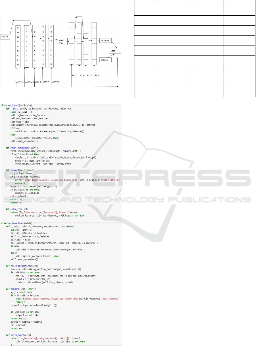
The architecture of convolutional neural networks

consists of the following layers (see Figure 1):

Convolution Layer

In the CNN architecture the purpose of extracting a

feature is done by a convolutional layer which has

two sets of operations (linear and nonlinear) defined

as activation function and convolutional operation.

Pooling Layer

In the CNN architecture, a feature map consists of

various number of dimensions to learn and perform

computation. The concept of pooling layer helps in

reduction of the dimensions of the feature maps so

minimal computation can be performed on the final

feature map.

Fully Connected Layer

Fully connected layers are known for connecting all

the inputs from upper layer to the activation units of

the lower layer. In each network the last few layers

will be fully connected layers so the extracted data

from all the upper layers will be compiled, and final

output is generated.

Figure 1: Update weights (Back Propagation).

3.2 Activation Functions

Activation functions are one of the most crucial parts

in the concept and design of neural networks. When the

activation function is chosen for a model, it defines the

model’s capability of learning the training datasets,

based on which the output predictions are made.

We have several types of activation functions are

below:

ReLu is known as Rectified Linear Activation

calculated by max (0.0, x). Here x is considered as an

input value, if x is negative then the activated function

returns an output of 0.0. In the case of x being positive

the output value is x.

Sigmoid is known as Sigmoid function calculated

by 1.0 / (1.0 + e

-x

). Outputs are in the range of [0, 1]. If

the input value is more towards the positive, then the

output is closer to 1.0 else the output is closer to 0.0.

Tanh known as Hyperbolic Tangent calculated by

– e

-x

) / (e

+ e

-x

). Outputs are in the range of -1 to

+ 1. If the input value is more towards the positive,

then the output is closer to +1.0 else the output is

closer to -1.0.

Fully Connected layers (FC) are placed at the end

of the architecture. They often function on an input

which is flattened and connected to all the neurons in

the network. To create a single feature vector, the

output generated by the convolutional layer is

flattened.

3.3 Forward and Backward

Propagations

In the forward propagation, starting with the input,

the computation goes through different hidden layers

and gets processed based on its activation function.

Once the input is processed, it is then passed to the

next consecutive layer in the forward direction.

Similarly backward propagation is performed.

Error calculations and weights adjustments are

propagated backwards to the previous layers. We

have output_vector and target_output_vector as an

input to backward propagation and

adjusted_weight_vector as an output.

ICEIS 2022 - 24th International Conference on Enterprise Information Systems

282

4 DOUBLE LAYER CNN

Figure 2: Skip layers implemented in architecture.

Figure 3: Code snippet for two linear functions.

# Model Avg loss

#Correct

prediction

Avg

Accuracy

1 0.693697 403/800 50.375

2 0.693474 403/800 50.375

3 0.693151 396/800 49.500

4 0.117733 780/800 97.500

5 0.018077 799/800 99.875

6 0.695256 401/800 50.125

7 0.015770 795/800 99.375

8 0.015053 798/800 99.750

Fig. 2 is the architecture diagram where the input is

directly sent to the 3

convolutional layer, skipping

first two layers. In the FC layers the data coming from

the FC1 layer is sent to the FC3 layer by skipping the

FC2 layer.

As the name says, we have developed 2 individual

layers linear 1, linear 2 and implemented these 2

different linear layers in the same model. We have

implemented 8 models: model 1 through model 8 as

follows.

Model 1 uses the inbuilt functions of the torch and

we have implemented the network using 5

convolutional layers and 4 fully connected layers.

After implementing the model, we have trained our

pre-processed dataset in the built model. After

training we tested the model with the test dataset. And

got the accuracy.

Here in model 2 we are skipped some of the layers

in convolutional and in the linear as well to see if

there is any improvement in the accuracy of the

model.

After implementing the model, we have trained

our pre-processed dataset in the built model. After

training we tested the model with the test dataset and

computed the accuracy.

Model 3 is implemented using the developed

functions; it hasn't used any inbuilt functions like in

model 1 and model 2. Here we have taken the source

code and changed the formula used in the linear

model and we used the changed formula in our model

3 and model 4 to see if there is any improvement in

the accuracy or not. We have developed the model

with 5 convolutional layers and 4 fully connected

layers. The data is sent to all the included layers i.e.,

data is passed to all 5 convolutional layers and 4 fully

connected layers. After implementing the model, we

have trained our pre-processed dataset in the built

model. After training we tested the model with the

test dataset.

DL-CNN: Double Layered Convolutional Neural Networks

283

Here in model 4, we are skipping some of the

layers in convolutional and in the linear as well to see

if there is any improvement in the accuracy of the

model. After implementing the model, we have

trained our pre-processed dataset in the built model.

After training we tested the model with the test

dataset. Finally, we have observed that model 4 has

better performance compared to other models. And

the model 3 also got better performance compared to

model 1 and model 2.

In model 5 we added multiple weights and

multiple bias values to each layer instead of addition

biases and we have sent this updates values of new

weights and bias to the next layers. We have trained

our pre-processed dataset in the built model and

tested the model with the test dataset.

Model 6 is implemented using the developed

functions; it hasn't used any inbuilt functions like in

model 1 and model 2. Here we have modified the

source code and changed the formula used in the

linear. The formula we used here is we added multiple

weights and multiple bias values to each layer and we

have sent this updates values of new weights and bias

to the next layers.

Model 7 we used separate functions and 2 separate

linear functions i.e., linear 1 and linear 2 and used

these 2 different linear functions in fully connected

layers. We have developed the model with 5

convolutional layers and 4 fully connected layers.

Model 8 is implemented using the developed

functions; it hasn't used any inbuilt functions like in

model 1 and model 2.

5 SIMULATIONS AND RESULTS

5.1 Datasets and Computer

The data set we used here is the 2 classes dataset that

has 4000 images of eyes open and closed of different

peoples and we extracted the data from online

resources (Patil, 2022). The computer used here is the

Alienware M17R3. It has an i7 processor,16GB

Ram,6GB Nvidia GeForce rtx2070 and has a storage

of 1TB SSD.

5.2 Results and Comparison

We ran our model with the data and the accuracy and

average loss of the model is observed. We can have

the loss for each batch of images is observed. You can

see the accuracy value i.e., (number of correct

images/total number of test images). Fig.

MODEL 1: - Accuracy

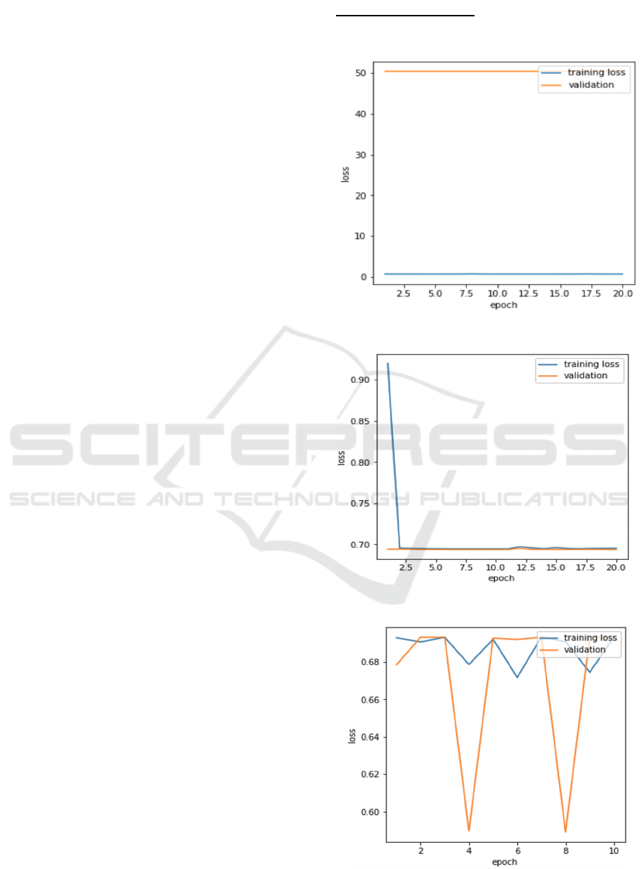
Graphical representation of the Loss value of batch

for the given epoch.

Figure 4: Loss Graph of Model 1.

Figure 5: Loss Graph of Model 2.

Figure 6: Loss Graph of Model 3.

ICEIS 2022 - 24th International Conference on Enterprise Information Systems

284

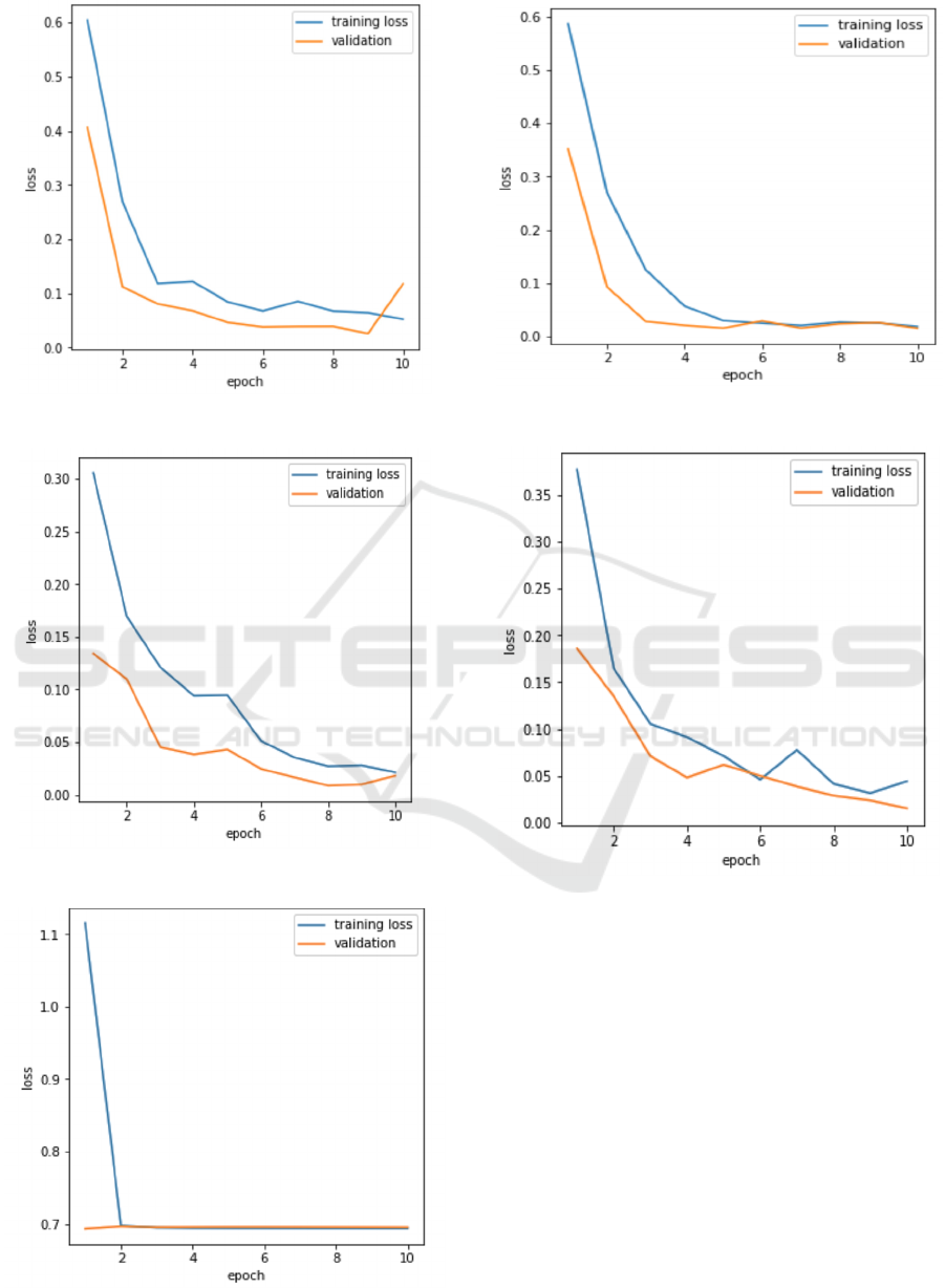
Figure 7: Loss Graph of Model 4.

Figure 8: Loss Graph of Model 5.

Figure 9: Loss Graph of Model 6.

Figure 10: Loss Graph of Model 7.

Figure 11: Loss Graph of Model 8.

6 CONCLUSIONS AND FUTURE

WORK

In the paper we proposed several new algorithms or

variations of CNN, including skipping layers, double

layers, multiplication biases, etc. Using the facial

datasets for classification, simulation results show

various degrees of improvements of the new

algorithms on the prediction accuracy over original

CNN algorithm.

In the future work we plan to change the padding

formula and stride values to check whether we can

further improve the performance and accuracy.

DL-CNN: Double Layered Convolutional Neural Networks

285

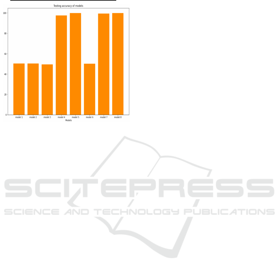
Overall Comparison of All the 8 Models

Figure 12: Accuracy Comparison of 8 models.

REFERENCES

Graves, A. e. (2009). A Novel Connectionist System for

Improved Unconstrained Handwriting Recognition.

IEEE Transactions on Pattern Analysis and Machine

Intelligence, 31 (5), 855–868.

Graves, A. M. (2013). Speech recognition with deep

recurrent neural networks. IEEE international

conference on acoustics, speech and signal processing,

(pp. 6645-6649).

He, K. e. (2016). Deep residual learning for image

recognition. Proceedings of the IEEE conference on

computer vision and pattern recognition.

Krizhevsky, A. (2012). ImageNet Classification with Deep

Convolutional Neural Networks. Advances in Neural

Information Processing Systems 25(2).

Lecun, Y. e. (1989). Backpropogation Applied to

Handwritten Zip Code Recognition. Neural

Computation 1, 541-551.

McCulloch, W. P. (1943). A logical calculus of the ideas

immanent in nervous activity. Bulletin of Mathematical

Biophysics 5, 115–133.

Patil, P. (2022). Retrieved from

https://www.kaggle.com/prasadvpatil/mrl-dataset

Rosenblatt, F. (1957). The Perceptron - A Perceving and

Recognizing Automaton. Buffalo: Cornell.

Rumelhart, D. H. (1986). Learning representations by back-

propagating errors. Nature 323, 533–536.

Simonyan, K. a. (2015). Very Deep Convolutional

Networks for Large-Scale Image Recognition. The 3rd

International Conference on Learning Representations

(ICLR2015), (pp. 1409-1556).

Tripathi, M. (2021). Analysis of convolutional neural

network based image classification techniques. Journal

of Innovative Image Processing (JIIP), 3(02), 100-117.

Wang, P. F. (2021). Comparative analysis of image

classification algorithms based on traditional machine

learning and deep learning. Pattern Recognition

Letters, 141,., 61-67.

Williams, R. J. (n.d.). .; Hinton, Geoffrey E.; Rumelhart,

David E. (October 1986). "Learning representations by

back-propagating errors". Nature. 323 (6088): 533–

536.

ICEIS 2022 - 24th International Conference on Enterprise Information Systems

286