Estimation of Looming from LiDAR

Juan D. Yepes and Daniel Raviv

Florida Atlantic University, Electrical Engineering and Computer Science Department,

Keywords:

Looming, Obstacle Avoidance, Collision Free Navigation, LiDAR, Threat Zones, Autonomous Vehicles.

Abstract:

Looming, traditionally deﬁned as the relative expansion of objects in the observer’s retina, is a fundamental

visual cue for perception of threat and can be used to accomplish collision free navigation. The measurement

of the looming cue is not only limited to vision and can also be obtained from range sensors like LiDAR

(Light Detection and Ranging). In this article we present two methods that process raw LiDAR data to es-

timate the looming cue. Using looming values, we show how to obtain threat zones for collision avoidance

tasks. The methods are general enough to be suitable for any six-degree-of-freedom motion and can be imple-

mented in real-time without the need for ﬁne matching, point-cloud registration, object classiﬁcation or object

segmentation. Quantitative results using the KITTI dataset shows advantages and limitations of the methods.

1 INTRODUCTION

Collision avoidance continues to be one of the great-

est challenges in unmanned vehicles (Yasin et al.,

2020) and autonomous driving (Roriz et al., 2021),

where the demand for increasingly robust, fast and

safe systems is crucial for the development of these

industries. It is closely tied with the perception of

threat. For creatures in nature, this task seems to

be more fundamental than the recognition of shapes

(Albus and Hong, 1990). Studies in biology have

shown strong evidence of neural circuits in the brains

of creatures related to the identiﬁcation of looming

(Ache et al., 2019). Basically, creatures have evolved

instinctive escaping behaviors that tie perception di-

rectly to action (Evans et al., 2018).

The visual looming cue, deﬁned quantitatively by

(Raviv, 1992) as the instantaneous change of range

over the range, is related to the increase in size of an

object projected on the observer’s retina. It is an indi-

cation of threat that can be used to accomplish colli-

sion avoidance tasks. The looming cue is not limited

exclusively to vision and can be computed from active

sensors like LiDAR (Light Detection and Ranging).

In general, architectures for autonomous vehi-

cles consist of three sub-systems: Perception, Plan-

ning and Control (Sharma et al., 2021). The Per-

ception sub-system can be divided subsequently into

three categories: camera-based, LiDAR-based and

sensor fusion-based approaches (Wang et al., 2018).

Traditionally the task of obstacle avoidance is ex-

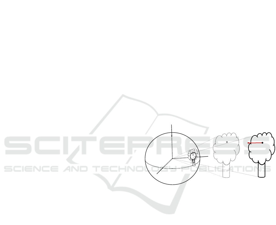
Figure 1: Visualizing looming cue: relative expansion of

3D object on 2D image sensor.

clusively related to the Planning and Control sub-

systems (Yasin et al., 2020) where classiﬁcation of

objects is a prerequisite prior to any global or local

path planning action (Mujumdar and Padhi, 2011).

In contrast, it has been shown that obstacle avoid-

ance tasks can be accomplished without 3D recon-

struction (structure from motion), using the Active

Perception paradigm (Aloimonos, 1992).

In this paper we follow an approach similar to (Ra-

viv and Joarder, 2000). It uses 2D raw data to directly

get quantitative indication of visual threat. We present

methods for obtaining looming values using raw Li-

DAR data and threat zones. This allows for real-time

collision avoidance tasks without 3D reconstruction

or scene understanding. In the proposed approach

further processing of the LiDAR point cloud is not

required for obtaining threat zones.

Yepes, J. and Raviv, D.

Estimation of Looming from LiDAR.

DOI: 10.5220/0011115300003191

In Proceedings of the 8th International Conference on Vehicle Technology and Intelligent Transport Systems (VEHITS 2022), pages 455-462

ISBN: 978-989-758-573-9; ISSN: 2184-495X

455

> >

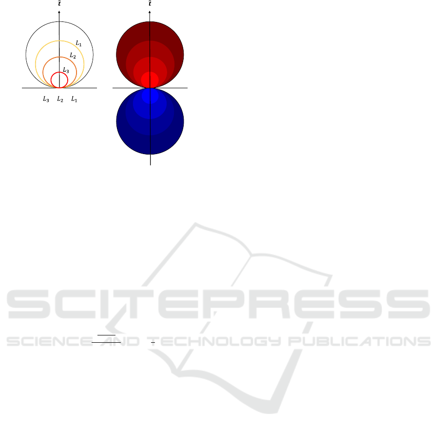
Figure 2: Equal looming spheres as shown in red for (L > 0)

and blue for (L < 0).

2 RELATED WORK

2.1 Visual Looming

The visual looming cue is related to the relative

change in size of an object projected on the observer’s

retina as the range to the object varies (Figure 1). It

is quantitatively deﬁned as the negative value of the

time derivative of the range between the observer and

a point in 3D divided by the range (Raviv, 1992):

L = − lim

∆t→0



−r

∆t



= −



˙r



(1)

where L denotes looming, dot denotes derivative

with respect to time.

2.1.1 Looming Properties

Note that the result for L in equation (1) is a scalar

value which is dependent on the vehicle translation

component but independent of the vehicle rotation.

It was shown that points in space around the vehi-

cle that share the same looming values form equal

looming spheres with centers that lie on the instan-

taneous translation vector t and intersect with the ve-

hicle origin. These looming spheres expand and con-

tract depending on the magnitude of the translation

vector (Raviv, 1992). Regions for obstacle avoidance

and other behavior related tasks can be deﬁned using

equal looming surfaces. For example, a high danger

zone for L > L

, medium threat for L

> L > L

and

low threat for L

> L > L

(Figure 2).

2.1.2 Advantages of Looming

Using the same LiDAR point cloud, it is possible to

get looming directly without 3D reconstruction and

without knowing the ego-motion of the LiDAR sen-

sor. Looming is measured in time

−1

units and pro-

vide information about imminent threat to the ob-

server. There is no need for scene understanding such

as identifying cars, bikes, or pedestrians. In addition,

looming provides threats for moving objects as well.

Extracting looming for obstacle avoidance using point

cloud raw data from LiDAR is the main contribution

of this paper.

2.1.3 Measuring Visual Looming

Several methods were shown to quantitatively extract

the visual looming cue on a 2D image sequence by

measuring attributes like area, brightness, texture den-

sity and image blur (Raviv and Joarder, 2000).

The Visual Threat Cue (VTC), just like the visual

looming, is a measurable time-based scalar value that

provides some measure for a relative change in range

between a 3D surface and a moving observer (Kundur

and Raviv, 1999).

Event-based cameras were shown to detect loom-

ing objects in real-time from optical ﬂow using clus-

tering of pixels (Ridwan, 2018).

2.2 LiDAR for Obstacle Avoidance

In general, collision avoidance approaches require

3D reconstruction of the environment where colli-

sion free paths can be computed an executed. Sev-

eral deep learning and path planning techniques for

autonomous driving were mentioned in (Grigorescu

et al., 2020). Point clouds, provided by LiDAR

sensors, are the preferred representation for many

scene understanding related applications. These point

clouds are processed to build real-time 3D local-

ization maps, using SLAM (Simultaneous Localiza-

tion and Mapping) and related techniques (Zhang and

Singh, 2014). In general, most methods use 3D object

detection, segmentation and scene understanding. In

addition, ego-motion is required for obstacle avoid-

ance and autonomous navigation.

In contrast, our approach provides relevant infor-

mation for the task of collision avoidance in the form

of a real-time looming threat map. This allows the di-

rect transition from perception to action without the

need of object identiﬁcation, ﬁnding ego-motion or

3D reconstruction.

VEHITS 2022 - 8th International Conference on Vehicle Technology and Intelligent Transport Systems

456

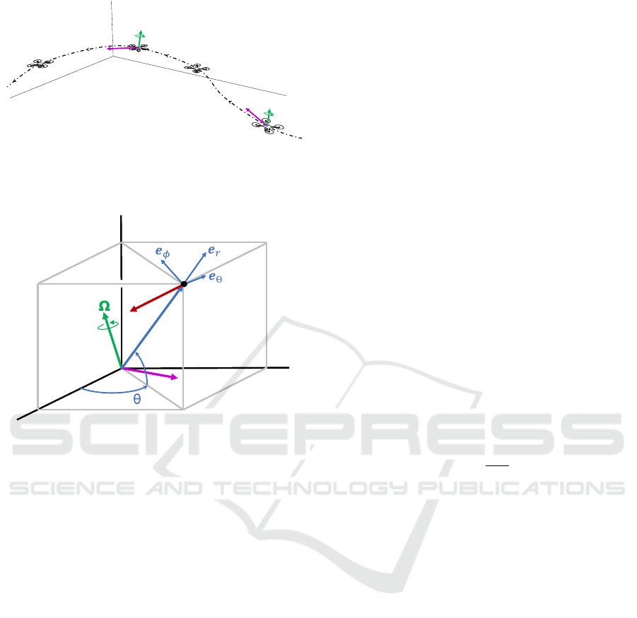
Figure 3: Vehicle undergoing a generalized six-degree-of-

freedom motion relative to the world frame. t is the transla-

tion velocity vector, and Ω is the rotation vector.

Figure 4: LiDAR coordinate system.

3 METHOD

3.1 Derivation of Looming from the

Relative Velocity Field

We will derive a general expression for Looming (L)

for any six-degree-of-freedom motion that involves

velocity and range using spherical coordinates. Then

we can apply this expression with LiDAR data.

Vehicle Motion. Consider a vehicle undergoing a

general six-degree-of-freedom motion in a 3-D space

relative to an arbitrary stationary reference point.

At any given time, the vehicle will have an associ-

ated translation velocity vector t and a rotation vector

Ω relative to the world frame as shown on Figure 3.

LiDAR Coordinate System. Consider a local coor-

dinate system centered at the LiDAR sensor, ﬁxed to

the moving vehicle. We chose the x-axis to be aligned

with the forward direction of the vehicle and the z-

axis to be aligned with the vertical orientation. Refer

to Figure 4: In this frame any stationary feature on the

3-D scene can be represented by spherical coordinates

(r, θ,φ) where r is the radial range to the feature point

F, θ is the azimuth angle measured from the x-axis

and φ is the elevation angle from the XY-plane.

Relative Velocity Field. In our analysis the vehicle

is undergoing a generalized six-degree-of-freedom

motion in the world frame. This is equivalent to in-

terpreting the motion as the vehicle being stationary

and the feature point F moving on the LiDAR frame

with opposite velocity vector −t and rotation −Ω.

In this LiDAR frame the feature F has relative ve-

locity vector:

V = (−t) + (−Ω × r) (2)

We can also conveniently express V using spherical

unit vector components e

, e

V = ˙re

+ r

θcos(φ)e

+ r

φe

(3)

Note that equations (2) and (3) refer to the same rela-

tive velocity ﬁeld V.(r in bold refers to the range vec-

tor and the scalar r to its magnitude, i.e r = |r|).

Looming from Normalized Velocity Field. We

can get another expression for looming (L) by divid-

ing equations (2) and (3) by r, expanding t and Ω, and

grouping components by e

L =

t · e

(4)

Notice that by knowing the instantaneous translation

vector of the vehicle t and range r, we can compute

the looming value (L) for any point along the direc-

tional unit vector e

3.2 Looming from LiDAR

We propose two ways to extract looming from LiDAR

data.

3.2.1 Using LiDAR Data Only

Looming can be estimated using LiDAR point clouds.

Each full scan of the LiDAR results in a range image

grid. Using two consecutive scans we get two range

image grids as obtained from the same 3D environ-

ment. Theoretically, if the range value of each LiDAR

pixel in each grid corresponds to the same 3D point

in space, we obtain two range values from which the

looming can be estimated, where the only error is due

to the range values as obtained from the LiDAR mea-

surements.

However, this is practically not the case: the prob-

lem with this approach is that due to the vehicle mo-

tion the assumption may hold only when the changes

Estimation of Looming from LiDAR

457

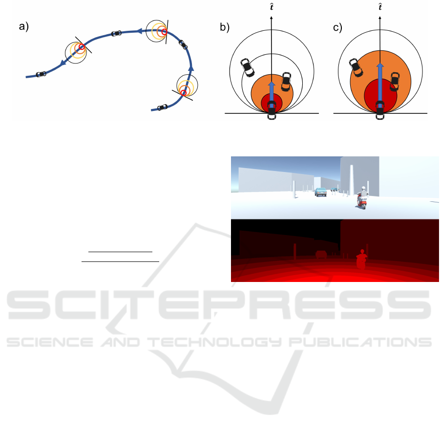
Figure 5: Equal looming circles. a) Vehicle trajectory, b) High and medium threat zones, c) Vehicle motion: higher speeds

results in an expansion of the threat region.

from one image to another are inﬁnitesimally small.

To minimize the effect of incorrect looming calcu-

lations and improve the robustness of the approach,

we use interpolation/decimation and discretization of

the data in the grid allowing for range values that are

closer to the real ones.

Equation (5) shows the speciﬁc calculations.

i j

= −



r(θ

,φ

)

j+1

−r(θ

,φ

)

∆t



r(θ

, φ

)

j+1

(5)

where i = [1, 2, .., n], n is the number of points on

the grid, j + 1, j correspond to the current and pre-

vious point cloud sample sets. The resulting L

i j

can

be interpreted as a LiDAR-based looming image from

where threat zones can be obtained for the purpose of

collision avoidance actions.

3.2.2 Using LiDAR + IMU

Another method for obtaining looming is using Li-

DAR and IMU (Inertial Measurement Unit). Even

though this is not the primary focus of this paper, its

purpose is to demonstrate that LiDAR combined with

IMU increase the robustness of computation of loom-

ing. However, this approach has its drawback because

it gives incorrect values of looming for moving ob-

jects. Note that it requires only the translation vector

and not the rotation component of the LiDAR sensor.

It uses ego-motion only partially, and there is no need

for 3D reconstruction and image understanding.

We can compute looming (L) for every measured

stationary point by using equation (4). The range r is

provided by the LiDAR sensor for every point on the

point cloud. The instantaneous translation vector t of

the vehicle can be obtained from the IMU or by other

odometry methods.

For special cases where vehicles have little side

motion, like most automotive applications, the trans-

lation vector can be assumed to be equal to the ve-

hicle forward motion component, and the magnitude

Figure 6: Looming from synthetic data: top image is the

scene; bottom image is the looming map (Brighter red rep-

resents higher value of looming).

(speed) can be obtained from the vehicle odometer or

from the speed encoder of the wheel.

3.2.3 Threat Maps

From either method, threat regions can be obtained

from looming values by assigning speciﬁc thresholds.

For example, High, Medium, or Low threat zones.

(Figure 5).

4 RESULTS

We present results of the methods for obtaining loom-

ing and threat zones using synthetic and real data.

4.1 Ground Truth Looming with

Synthetic Data

A simulation of a moving vehicle in a stationary en-

vironment was performed using the Unity3D game

engine. In this simulation the vehicle is translating

forward at a constant speed between some stationary

objects. The top part of Figure 6 shows an actual im-

age of the scene. The bottom part of Figure 6 shows

VEHITS 2022 - 8th International Conference on Vehicle Technology and Intelligent Transport Systems

458

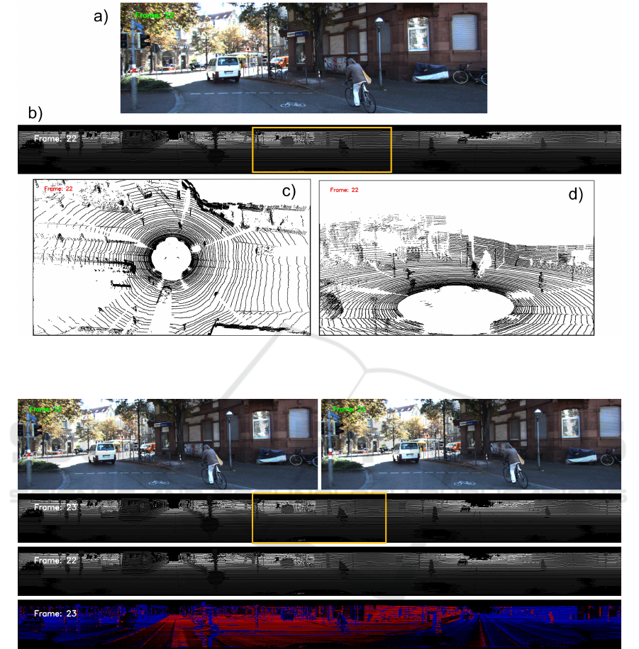
Figure 7: LiDAR data from the KITTI dataset: a) Original image from a color camera mounted on the vehicle, b) 360 degrees

LiDAR data, the yellow rectangle corresponds to the color camera ﬁeld of view, c) Top view of point cloud in 3D, d) Bird’s

eye 3D view of point cloud.

Figure 8: Estimated looming from LiDAR only. (Refer to text for details).

ground truth looming computed using equation (1)

and shown from the observer point of view. A pixel

shader ﬁlter was implemented to visualize the loom-

ing value as levels of red color. Brighter red color

corresponds to higher value of looming.

4.2 LiDAR Data from KITTI Dataset

We processed real data using a particular city drive

from the well-known KITTI dataset (Geiger et al.,

2013). The KITTI dataset includes raw data provided

by a Velodyne 3D laser scanner (LiDAR) along with

velocity vector from a GPS/IMU inertial navigation

system. Color camera images were only used as ref-

erence as shown in Figure 7.a. The LiDAR sensor

speciﬁcations are: Velodyne HDL-64E rotating 3D

laser scanner, 10 Hz, 64 beams, 0.09-degree angular

resolution, 2 cm distance, accuracy, provides around

1.3 million points/second, ﬁeld of view: 360 degrees

horizontal, 26.8 degrees vertical, range:120 m.

Shown in Figure 7 are the original images from

one of the vehicle color cameras and gray-scale rep-

resentations of the raw LiDAR data. A yellow rectan-

gle indicates where the LiDAR data matches the ﬁeld

Estimation of Looming from LiDAR

459

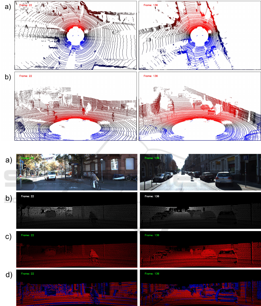
Figure 9: Looming from LiDAR (red is potential threat): a) Top view, b) Bird’s eye view.

Figure 10: Looming from Lidar: a) Original image, b) Depth from LiDAR, c) Looming from LiDAR + IMU, d) Estimated

looming from LiDAR only.

of view of the color camera. Also shown are top and

bird’s eye views of the data for a speciﬁc time instant

of the video.

4.3 Estimation of Looming using

LiDAR

In Figure 8, original images from two consecutive

frames (frames 22 and 23) are shown along LiDAR

VEHITS 2022 - 8th International Conference on Vehicle Technology and Intelligent Transport Systems

460

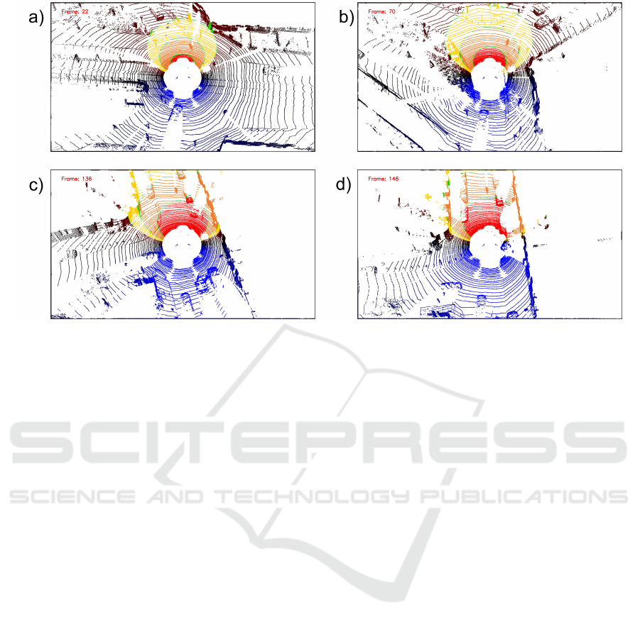
Figure 11: Threat zones expanding and contracting according to looming (refer to text for details).

views (360 degrees) for two time instants. The re-

sultant looming estimation using equation (5) is also

shown at the bottom of Figure 8. Notice positive

values of looming are shown in red and corresponds

mainly to points along the forward direction of mo-

tion (around the center of the image).

Due to the effect of occlusions of points, there are

sudden changes in range between frames, causing an

”edge-effect” around objects with incorrect looming

values, shown in intense red or blue colors. However

an important advantage is that the method incorpo-

rates values of looming as obtained from moving ob-

jects. For example, the bicycle in the middle of the

image is correctly portrayed with dark colors, mean-

ing low values of looming as expected for this kind of

motion since the bicycle velocity almost matches the

velocity of the vehicle, and the rate of change in range

is close to zero.

4.4 Looming from LiDAR and IMU

We use equation (4) to compute looming for each

point. From the IMU sensor we obtained the trans-

lation velocity vector t and from the LiDAR sensor

we obtained the range r. Figure 9 shows top and

bird’s eye views for two time instants. Color intensity

was assigned to each point representing the obtained

looming value: red for positive values, and blue for

negative values.

We can see that the looming is very similar to

the expected shown in simulation. This method ade-

quately registers looming for stationary objects; how-

ever, it is imprecise for moving objects since the rela-

tive speed is not considered.

In Figure 10 a comparison between both methods

is shown.

4.5 Threat Zones for Collision Free

Navigation

In Figure 11 several threat zones are computed us-

ing looming from section 4.4: red zone - high threat,

orange zone - medium threat and yellow zone - low

threat. Notice how the threat zones change sizes be-

tween frames, this is due to the change in speed of the

vehicle.

5 CONCLUSIONS

In this paper we demonstrate how to compute loom-

ing directly from raw LiDAR data without 3D recon-

struction. There is no need for scene understanding

such as identifying cars, bikes, or pedestrians. Two

approaches are shown, one uses LiDAR data only, and

the other uses LiDAR data combined with IMU.

The approach shows that looming provides infor-

mation about imminent threat that can potentially be

used for navigation tasks such as obstacle avoidance.

The paper shares highly encouraging initial results

and should be considered as “work in progress” as

more looming from LiDAR-related methods are be-

ing explored.

Estimation of Looming from LiDAR

461

ACKNOWLEDGEMENTS

The authors thank Dr. Sridhar Kundur for many fruit-

ful discussion and suggestions that led to meaningful

improvements of this manuscript.

REFERENCES

Ache, J. M., Polsky, J., Alghailani, S., Parekh, R., Breads,

P., Peek, M. Y., Bock, D. D., von Reyn, C. R., and

Card, G. M. (2019). Neural basis for looming size and

velocity encoding in the drosophila giant ﬁber escape

pathway. Current Biology, 29(6):1073–1081.

Albus, J. S. and Hong, T. H. (1990). Motion, depth, and im-

age ﬂow. In Proceedings., IEEE International Confer-

ence on Robotics and Automation, pages 1161–1170.

IEEE.

Aloimonos, Y. (1992). Is visual reconstruction necessary?

obstacle avoidance without passive ranging. Journal

of Robotic Systems, 9(6):843–858.

Evans, D. A., Stempel, A. V., Vale, R., Ruehle, S., Leﬂer,

Y., and Branco, T. (2018). A synaptic threshold

mechanism for computing escape decisions. Nature,

558(7711):590–594.

Geiger, A., Lenz, P., Stiller, C., and Urtasun, R. (2013).

Vision meets robotics: The kitti dataset. The Inter-

national Journal of Robotics Research, 32(11):1231–

1237.

Grigorescu, S., Trasnea, B., Cocias, T., and Macesanu,

G. (2020). A survey of deep learning techniques

for autonomous driving. Journal of Field Robotics,

37(3):362–386.

Kundur, S. R. and Raviv, D. (1999). Novel active vision-

based visual threat cue for autonomous navigation

tasks. Computer Vision and Image Understanding,

73(2):169–182.

Mujumdar, A. and Padhi, R. (2011). Evolving philoso-

phies on autonomous obstacle/collision avoidance of

unmanned aerial vehicles. Journal of Aerospace Com-

puting, Information, and Communication, 8(2):17–41.

Raviv, D. (1992). A quantitative approach to looming. US

Department of Commerce, National Institute of Stan-

dards and Technology.

Raviv, D. and Joarder, K. (2000). The visual looming nav-

igation cue: A uniﬁed approach. Comput. Vis. Image

Underst., 79:331–363.

Ridwan, I. (2018). Looming object detection with event-

based cameras. University of Lethbridge (Canada).

Roriz, R., Cabral, J., and Gomes, T. (2021). Automotive

lidar technology: A survey. IEEE Transactions on In-

telligent Transportation Systems.

Sharma, O., Sahoo, N. C., and Puhan, N. (2021). Recent

advances in motion and behavior planning techniques

for software architecture of autonomous vehicles: A

state-of-the-art survey. Engineering applications of

artiﬁcial intelligence, 101:104211.

Wang, M., Voos, H., and Su, D. (2018). Robust online ob-

stacle detection and tracking for collision-free navi-

gation of multirotor uavs in complex environments.

In 2018 15th International Conference on Control,

Automation, Robotics and Vision (ICARCV), pages

1228–1234. IEEE.

Yasin, J. N., Mohamed, S. A., Haghbayan, M.-H., Heikko-

nen, J., Tenhunen, H., and Plosila, J. (2020). Un-

manned aerial vehicles (uavs): Collision avoidance

systems and approaches. IEEE access, 8:105139–

105155.

Zhang, J. and Singh, S. (2014). Loam: Lidar odometry

and mapping in real-time. In Robotics: Science and

Systems, volume 2, pages 1–9. Berkeley, CA.

VEHITS 2022 - 8th International Conference on Vehicle Technology and Intelligent Transport Systems

462