Impact of Hyperparameters on the Generative Adversarial Networks

Behavior

Bihi Sabiri

1 a

, Bouchra El Asri1

and Maryem Rhanoui

2 c

IMS Team, ADMIR Laboratory, Rabat IT Center, ENSIAS, Mohammed V University in Rabat, Morocco

Meridian Team, LYRICA Laboratory, School of Information Sciences, Rabat, Morocco

Keywords:

Recommendation Systems, Machine Learning, Deep Learning, Neural Network, Generative Adversarial

Networks.

Abstract:

Generative adversarial networks (GANs) have become a full-ﬂedged branch of the most important neural

network models for unsupervised machine learning. A multitude of loss functions have been developed to train

the GAN discriminators and they all have a common structure: a sum of real and false losses which depend

only on the real losses and generated data respectively. A challenge associated with an equally weighted sum

of two losses is that the formation can beneﬁt one loss but harm the other, which we show causes instability

and mode collapse. In this article, we introduce a new family of discriminant loss functions which adopts a

weighted sum of real and false parts. With the use the gradients of the real and false parts of the loss, we

can adaptively choose weights to train the discriminator in the sense that beneﬁts the stability of the GAN

model. Our method can potentially be applied to any discriminator model with a loss which is a sum of the

real and fake parts. Our method consists in adjusting the hyper-parameters appropriately in order to improve

the training of the two antagonistic models Experiences validated the effectiveness of our loss functions on

image generation tasks, improving the base results by a signiﬁcant margin on dataset Celebdata.

1 INTRODUCTION

Generative Adversarial Networks (GAN) (Goodfel-

low et al., 2020) technology, is an innovative pro-

gramming approach for building generative models,

that are, models capable of producing data on their

own (Brownlee, 2020) (Parthasarathy et al., 2020).

The GAN (Abdollahpouri et al., 2020) rapid devel-

opment in recent years and its multiple applications

make it one of the most promising recent discover-

ies in machine learning. Yann LeCun (head of AI re-

search at Facebook) has also presented it as ”the most

interesting idea of the last 10 years in the ﬁeld of Ma-

chine Learning” (Rocca, 2021).

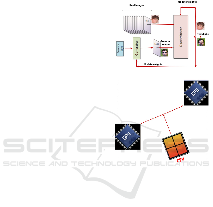
In technical terms, GANs are based on the un-

supervised learning of two artiﬁcial neural networks

called Generator and Discriminator. These two net-

works train each other in a contradictory relationship

using convolutional layers (Barua S et al., 2019) (Sun

H et al., 2020): The Generator is in charge of creating

designs (ex: images), the Discriminator receives de-

https://orcid.org/0000-0003-4317-568X

https://orcid.org/0000-0001-8502-4623

https://orcid.org/0000-0002-0147-8466

signs from the generator and from a database of actual

designs. As a result of the Discriminator’s work, two

feedback loops convey to the two neural networks the

identity of the designs on which they need to improve.

The Generator receives the identity of the designs on

which it has been unmasked by the Discriminator, The

Discriminator receives the identity of the designs on

which it has been deceived by the Generator.

The two algorithms therefore maintain a win-win

relationship of continuous improvement: the Genera-

tor learns to create increasingly realistic designs and

the Discriminator learns to better and better identify

the real designs from those coming from the Genera-

tor.

There are many applications in industry. Automo-

tive manufacturers are particularly interested in GAN

to sharpen images captured by autonomous vehicle

cameras and thus improve the efﬁciency of artiﬁcial

vision algorithms. In the construction sector, for ex-

ample, a GAN has been used to simulate the activity

of future occupants of a building and thus feed sim-

ulation algorithms aimed at optimizing energy con-

sumption as accurately as possible. Finally, GANs

have already been implemented in the fashion sec-

428

Sabiri, B., El Asri, B. and Rhanoui, M.

Impact of Hyperparameters on the Generative Adversarial Networks Behavior.

DOI: 10.5220/0011115100003179

In Proceedings of the 24th International Conference on Enterprise Information Systems (ICEIS 2022) - Volume 1, pages 428-438

ISBN: 978-989-758-569-2; ISSN: 2184-4992

tor to design shoes or fabrics that will appeal to con-

sumers. With this ability to imitate without actually

copying, GANs could have far-reaching implications

for industrial design and copyright protection.

With regard to the limitations of the command sys-

tems, namely: sparsity and noise, two lines of re-

search have were conducted, and their common ideas

can be summarized as follows:

1. For the problem of data sparsity, data augmenta-

tion (Sandy et al., ) implemented by capturing the

distribution of real data under the minimax is the

main adaptation strategy.

2. For the issue of data noise, adversarial distur-

bances and training based on adversarial sampling

are often used as a solution (Mayer and Timofte,

2020).

In this article, we will take a closer look at GANs

and the different variations to their loss functions

(Brownlee, 2020), so that we can get a better insight

into how the GAN works while addressing the unex-

pected performance issues. The standard GAN loss

function, also known as the min-max loss (Brown-

lee, 2020),will be used to train these two models. The

generator tries to minimize this function while the dis-

criminator tries to maximize it. The rest of this paper

is organized as follows. In Section 2 we brieﬂy com-

pare and position our solution with other proposals

ﬁnd in the literature. Section 3 describes the prob-

lem handled. In Section 4, we describe our proposed

method that can be potentially applied to any discrim-

inator model with a loss that is a sum of the real and

fake parts.

2 STATE-OF-THE-ART

The Generative Adversarial Networks refers to a fam-

ily of generative models that seek to discover the un-

derlying distribution behind a certain data generating

process. It is described as two models in competition

which, when trained, is able to generate samples in-

discernible from those sampled from the normal dis-

tribution This distribution is discovered through an

adversarial competition between a generator and a

discriminator. The two models are trained such that

the discriminator strives to distinguish between gen-

erated and true examples, while the generator seeks

to confuse the discriminator by producing data that

are as realistic and compelling as possible. This gen-

erative model puts in competition two networks of

neurons D and G which will be called hereafter the

discriminator and the generator, respectively. In this

section, we present a brief review of existing litera-

ture of generative adversarial networks. In this study

(Goodfellow et al., 2020) (Mao and Li, 2021), GANs

were formulated for the ﬁrst time. This article demon-

strates the potential of GANs as a generative model.

GANs became popular for image synthesis based on

the successful use of deep convolution layers (Mao

and Li, 2021) (noa, 2015).

Classical Algorithms. Classical image processing

algorithms are unsupervised algorithms that improve

low-light images through well-founded mathematical

models. They are efﬁcient and simple in terms of cal-

culation. But they are not robust enough and require

manual calibration to be used in certain conditions

(Tanaka et al., 2019).

Implicit Model for Generation. Apart from the

descriptive models, another popular branch of deep

generative models are black-box models which map

the latent variables to signals via a top-down CNN,

such as the Generative Adversarial Network (GAN)

(Goodfellow et al., 2020) and its variants. These mod-

els have gained remarkable success in generating re-

alistic images and learn the generator network with an

assistant discriminator network.

Adversarial Networks. Generative Adversarial Net-

work (Goodfellow et al., 2020) have proven to per-

form sufﬁciently well for many supervised and un-

supervised learning problems. In (Zhu et al., 2017)

the authors propose a model through which the need

for paired images has been elevated and image trans-

lation between two domains can be done through

cycle-consistence loss. These techniques have been

applied to many other applications including dehaz-

ing, super-resolution, etc. Lately, it has been applied

to low light image enhancement in EnlightenGAN

(Jiang et al., 2019) with promising results and this

has motivated our GAN model. Generative adver-

sarial networks (Goodfellow et al., 2020) have also

beneﬁted from convolutional decoder networks, for

the generator network module. Denton et al (Denton

et al., 2015) used a Laplacian pyramid of adversar-

ial generator and discriminators to synthesize images

at multiple resolutions. This work generated com-

pelling high-resolution images and could also condi-

tion on class labels for controllable generation. Rad-

ford (Alec et al., 2015) used a standard convolutional

decoder, but developed a highly effective and stable

architecture incorporating batch.

Fully Connected GANs. The ﬁrst GAN architec-

tures used fully connected neural networks for both

the generator and discriminator (Goodfellow et al.,

2020). This type of architecture was applied to rela-

tively simple image data sets: Kaggle MNIST (hand-

written digits), CIFAR-10 (natural images), and the

Toronto Face Data Set (TFD).

Impact of Hyperparameters on the Generative Adversarial Networks Behavior

429

3 PROBLEM DESCRIPTION

In this article we will make a comparative study be-

tween two methods of calculating the loss: the ﬁrst

consists in calculating this loss globally on the gener-

ator and the desciminator and comparing it to that of

the descriminator with some hyper-parameters (Fig-

ure 1). The second consists in summing the losses of

the two antagonistic models with trying to to ﬁnd the

optimal hyper-parameters (Figure 1).

The discriminator network consists of convolu-

tional layers. For every layer of the network, we are

going to perform a convolution, then we are going

to perform batch normalization to make the network

faster and more accurate and ﬁnally, we are going to

perform a Leaky ReLu.

As for the generator, we’re going to give it a noise

vector, it’s going to be numbers generated as a vector

of 100 of numbers between -1 and 1 drawn randomly

according to a normal distribution, it’s really noise,

and in output the generator produces an image which

will be of the same geometry as the image which is

good with deconvolution processing to make a pro-

cessing equivalent to the processing of the discrimi-

nator then we went back in the other direction to gen-

erate generate deconvolution processing weights.

Here we are going to start from a small vector, a

vector 100 which is going to be a noise vector and

we are going to gradually recreate an image of the

same geometry as that which is taken as input to the

discriminator. The question now is how to train this

generator. We have a neural network that provides us

with an output, what we would like is that the output

is generally something else even if in the long term

after learning we would like that the neural network

gives us the output that we expect. But we always

have a difference between what we would like to have

and what we really have from the neural network. So

from this difference we creates a loss function and

by calculating the gradient on this loss function we

can then correct the weights of our neural network.

The loss calculation will be made on the generator

and discriminator assembly. This is how we will then

be able to then, after having calculated the gradient of

the whole, we will be able to correct the variables of

the generator and the discriminator.

GANs require higher computing power and the in-

frastructure is at the same level. When using GANs,

you need to have more data trafﬁc because these mod-

els will be very large and there are many parame-

ters, so training requires a lot of computing power and

memory (Figure 2).

Figure 1: GAN Backpropagation.

Figure 2: Good GANs with a good saddle.

4 THEORICALS RESULTS

4.1 Gradient Descent

The generator G implicitly deﬁnes a probability dis-

tribution p

as the distribution of the samples G(z)

obtained when z ∼ p

. Therefore, we would like al-

gorithm 1 to converge to a good estimator of p

data

, if

given enough capacity and training time. The results

of this section are done in a nonparametric setting,

e.g. We represent a model with inﬁnite capacity by

studying convergence in the space of probability den-

sity functions We will show in section 2.5 that this

minimax game has a global optimum for p

= p

data

4.2 Discriminator

The goal of the discriminator is to correctly label the

real images as true and generated images as false (see

Figure 3). Therefore, we might consider the following

to be the loss function of the discriminator:

ICEIS 2022 - 24th International Conference on Enterprise Information Systems

430

Algorithm 1: Minibatch stochastic gradient descent training

of generative adversarial nets. The number of steps to apply

to the discriminator, k, is a hyperparameter. We used k = 1,

the least expensive option, in our experiments (Goodfellow

et al., 2020).

for number of training iterations do for k steps do for

k steps do

1. Sample minibatch of m noise samples z (1) , . . . , z

(m) from noise prior pg(z).

2. Sample minibatch of m examples x (1) , . . . , x (m)

from data generating distribution pdata(x).

3. Update the discriminator by ascending its stochastic

gradient:

∇

θd

∑

i=1

[log



D(x

(i)

)



+ log



1 − D(G(z

(i)

))



]

4. end for

Sample minibatch of m noise samples z (1) , . . . , z

(m) from noise prior pg(z). Update the generator by

descending its stochastic gradient:

∇

θg

∑

i=1

[log



1 − D(G(z

(i)

))



]

5. end for

The gradient-based updates can use any standard gradient-

based learning rule. We used momentum in our experi-

ments.

Note: There is sometimes an analogy in the literature to the

falsiﬁcation of works of art. D is then called the ”critic” and

G is called the ”forger”. The objective of G is to transform a

random noise z into a sample ˆx as similar as possible to the

real observations x ∈ X. Conversely, the goal of D is to learn

to recognize ”false” samples ˆx from true observations x. The

GAN loss function (Brophy et al., 2021) will be presented as a

mathematical equation to show how the network is functioning

and how the error is calculated and propagated to update the

parameters to achieve different goals in the network.(This ex-

planation is heavily inspired and based on (Goodfellow et al.,

2020) and (Rome, 2017).

Discriminator

Generator

D(x) : To maximize D(G(z)) : To maximize

D(G(z)) : To minimize

Figure 3: Objective of two models.

= Error(D(x), 1) +

Error(D(G(z)), 0) (a)

Here, we are using a very generic, unspeciﬁc nota-

tion for Error to refer to some function that tells us the

distance or the difference between the two functional

parameters.

4.3 The Generator

The goal of the generator is to confuse the discrim-

inator as much as possible such that it mislabels

generated images as being true (see Figure 3).

= Error(D(G(z)),1) (b)

The key here is to remember that a loss func-

tion is something that we wish to minimize. In the

case of the generator, it should strive to minimize

the difference between 1, the label for true data, and

the discriminator’s evaluation of the generated fake

data. A common loss function that is used in binary

classiﬁcation problems is binary cross entropy. The

formula for cross entropy looks like (Tae, 2020):

H(p, q) = E

x∼p

data

(x)

[−logq(x)] (1)

In classiﬁcation tasks, the random variable is dis-

crete. Hence, the expectation can be expressed as a

summation.

H(p, q) = −

∑

x=1

p(x)log(q(x)) (2)

I the case of binary cross entropy, since there are

only two labels: zero and one. So the equation 2 can

be expressed as:

H(y, ˆy) = −

∑

ylog( ˆy) +(1 −y)log(1 − ˆy) (3)

This is the Error function that we have been

loosely using in the sections above. Binary cross

entropy fulﬁls our objective in that it measures how

different two distributions are in the context of binary

classiﬁcation of determining whether an input data

point is true or false. Applying this to the loss

functions in equation 3, we obtain:

= −

∑

x∈χ,z∈ζ

log(D(x)) + log(1 − D(G(z))) (4)

We can do the same for equation 2:

= −

∑

x∈χ,z∈ζ

log(D(G(z))) (5)

Impact of Hyperparameters on the Generative Adversarial Networks Behavior

431

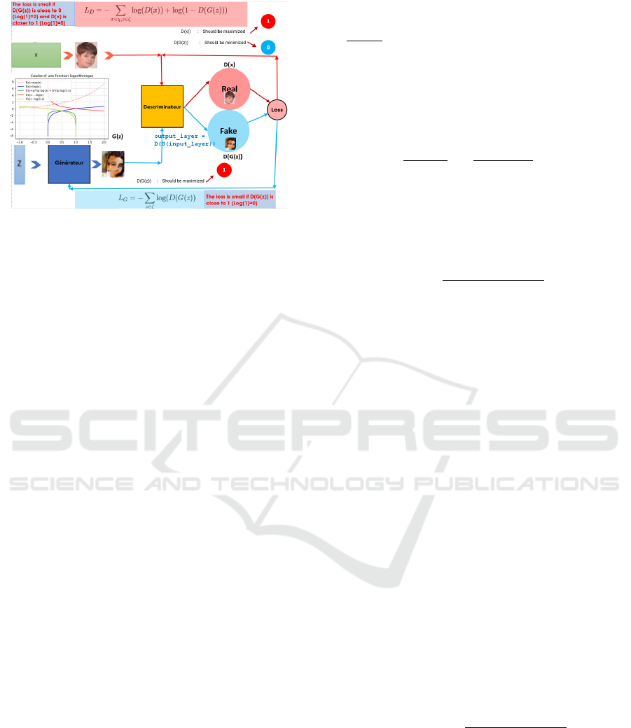
Figure 4: Generator & Discriminator functions loss.

4.4 Model Optimization

Now that we have deﬁned the loss functions for gener-

ator and discriminator, it is time to take advantage of

the math to solve the optimization problem, i.e. ﬁnd

the parameters for generator and discriminator such

as loss functions are optimized. This corresponds to

the formation of the model in practical terms.

4.5 The Discriminator Cost

Conceptually, the goal of learning is to maximize the

expectation that the discriminator, D, correctly cate-

gorizes the data as either real or fake. The goal of

learning for the generator, G, is to fool the discrimi-

nator.

When training a GAN, we usually train one model

at a time (Figure 4). In other words, when learning the

discriminator, the generator is assumed to be ﬁxed.

Mathematically, the goal of learning is to minimize

the following objective function:

min

max

V (G,D) = min

max

x∼p

data

(x)

[logD(x)]+

z∼p

generated

(z)

[1 − logD(G(z))]

(6)

In reality, we are more interested in the distribu-

tion modeled by the generator than in p

. Therefore,

let’s create a new variable, y = G(z), and use this sub-

stitution to rewrite the value function in (Equation 6):

min

max

V (G,D) = min

max

x∼p

data

(x)

[logD(x)]

z∼p

generated

(z)

[1 − logD(y)]

(7)

x∈χ

data

(x)log(D(x)) + p

(x)log(1 − D(x))dx

(8)

For ll (a, b) ∈ (R

∗

), the function y→a ∗

log(y) + b ∗ log(1 − y) achieves its maximum in [0,1]

a + b

The purpose of the discriminator is to maximize

the value of this Function 8. By a partial derivative

of V (G,D) with respect to D(x) see equation 8 , we

see that the optimal discriminator, noted D*(x), oc-

curs when the derivative with respect to D(x) is zero:

data

(x)

D(x)

(x)

(1 − D(x))

= 0 (9)

The optimum point is where the discriminator

fails to differentiate between the real input and the

synthesized data. For a ﬁxed Generator, the optimal

discriminator D is, (by simplifying Equation 9):

∗

(x) =

data

(x)

data

(x) + p

(x))

(10)

For G ﬁxed, this is the condition of the optimal dis-

criminator ! Note that the formula makes intuitive

sense: if a sample x is very authentic, we would ex-

pect p

data

(x) to be close to 1 and p

(x) to converge to

zero, in which case the optimal discriminator would

assign 1 to that sample. (D(x) = 1) which corre-

sponds to the label of the real images. In contrast,

for a generated sample x = G(z), we would expect the

optimal discriminator to assign a label of zero, since

data

(G(z)) must be close to zero.

4.6 The Generator Cost

To train the generator, we assume the discriminator

is ﬁxed and analyze the value function. Let’s start by

plugging the result we found above, namely (equation

10), into the value function to see what happens.

Note that the training objective for D can be in-

terpreted as maximizing the log-likelihood for

estimating the conditional probability P(Y = ykx),

where Y indicates whether x comes from p

data

(with

y = 1) or from p

(with y = 0). From (equation 10)

we can deduce:

1 − D

∗

(x) =

(x)

data

(x) + p

(x))

(11)

The minimax game in Equation 6 can now be refor-

mulated as:

ICEIS 2022 - 24th International Conference on Enterprise Information Systems

432

C(G) = max

V (G,D

∗

) = E

x∼p

data

(x)

[logD

∗

(x)]

z∼p

generated

(z)

log[1 − D

∗

(y)]

= E

x∼p

data

(x)

[log

data

(x)

data

(x) + p

(x))

]

x∼p

generated

(x)

[log

(x)

data

(x) + p

(x))

]

(12)

To proceed from here, we need a little inspiration.

Theorem 1.

The global minimum of the virtual learning criterion

C(G) = maxV(G,D)= V(G,D*) is reached if and only

if p

= p

data

. At this point, C(G) reaches the value

−log(4). (Goodfellow, 2016)

C(G) = −log(4) + D

data

(x) + p

(x)

)

data

(x) + p

(x)

)

(13)

where KL is the Kullback–Leibler divergence.

We recognize in the previous expression the Jensen–

Shannon divergence between the model’s distribution

and the data generating process:

C(G) = −log(4) + 2JSD(p

data

||p

) (14)

We recognize in the previous expression the

Jensen–Shannon divergence between two distribu-

tions (the distribution of the model and the process

of data generation) which is always non-negative, and

zero if they are equal, we have shown that C

∗

−log(4) is the global minimum of C(G) and that the

only solution is p

= p

data

, i.e., the generative model

perfectly replicating the data distribution. Basically

what is happening is that we are exploiting the prop-

erties of logarithms to extract a -log4 that did not ex-

ist before. In extracting this number, we inevitably

apply changes to the terms of expectation, including

dividing the denominator by two. Why was this nec-

essary? The magic here is that we can now interpret

the expectations as a Kullback-Leibler divergence:

The conclusion of this analysis is simple: the goal

of learning the generator, which is to minimize the

value function V(G,D), we want the JS divergence be-

tween the distribution of the data and the distribution

of the generated examples to be the smaller possible.

This conclusion certainly ﬁts our intuition: we want

the generator to be able to learn the underlying distri-

bution of the data from sampled training examples. In

other words, p

and p

data

should be as close to each

other as possible. The optimal generator G is there-

fore the one which is able to mimic p

data

to model a

convincing model distribution p

4.7 Loss Function

The loss function described in the original paper by

Ian Goodfellow et al. can be derived from the formula

of binary cross-entropy loss (equation 2). The binary

cross-entropy loss can be written as,

L(y, ˆy) = −

∑

i=1

log( ˆy

) (15)

In binary classiﬁcation, where the number of

classesN

equals 2, cross-entropy can be calculated

as:

L(y, ˆy) = −(y log(

y) + (1 − y)log(1 − ˆy)) (16)

4.7.1 Discriminator Loss

While training discriminator, the label data coming

from P

data

(x) is y=1 (real data) and

y=D(x) , By sub-

stitution of this in the loss function above (Equation

16), we get:

L(D(x), 1) = log(D(x)) (17)

Conversely, for data coming from generator, the label

is y=0 (fake data) and

y=D(G(z)). So from equation

16 the loss in this case is:

L(D(G(z)),0) = log(1 − D(G(z))) (18)

Now, the objective of the discriminator is to

correctly classify the fake and real dataset. For this,

equations (1) and (2) should be maximized and ﬁnal

loss function for the discriminator can be given as,

(D)

= max[log(D(x)) +log(1 − D(G(z)))] (19)

4.7.2 Generator Loss

The generator is competing against discriminator.

So, it will try to minimize the equation (3) and loss

function is given as:

(G)

= min[log(D(x)) + log(1 − D(G(z)))] (20)

Impact of Hyperparameters on the Generative Adversarial Networks Behavior

433

4.7.3 Combined Loss Function

We can combine equations (3) and (4) and write as:

L = min

max

[log(D(x))+log(1− D(G(z)))] (21)

Remember that the above loss function is valid

only for a single data point, to consider entire dataset

we need to take the expectation of the above equation

as:

min

max

V(G,D) = min

max

x∼p

data

(x)

[logD(x)]

z∼p

generated

(z)

[1 − logD(G(z))]

(22)

which is the same equation as described above

(see equation 6).

4.8 Experimental Setup

The two main types of networks to construct are either

Deep Convolutional GANs (DC-GANs) or fully con-

nected (FC) GANs. Which you use will depend on

the training data you are submitting to the network.

If you are using single data points, an FC network is

more appropriate, and if you are using images, a DC-

GAN is more appropriate (Stewart, ). In this paper we

will use the second type. We trained adversarial nets

on an a range of datasets including CELEBA (Jes-

sica, ),which consists of over 63,000 cropped anime

faces, and evaluate adversarial nets on the following

two tasks.

4.8.1 First Scenario

The generator nets used a mixture of rectiﬁer linear

activations (Jarrett et al., 2009) and tanh activations,

while the discriminator net used sigmoid activations.

Dropout was applied and other noise at intermediate

layers of the generator, we used noise as the input to

only the bottommost layer of the generator network.

Note that generative modeling is an unsupervised

learning task, so the images do not have any labels.

The input to the generator is typically a vector or a

matrix of random numbers (referred to as a latent ten-

sor) which is used as a seed for generating an image.

The generator will convert a latent tensor of shape

(100, 1, 1) into an image tensor of shape 4 x 4 x 128.

Both latent tensor (z) and a matrix for real images are

mapped to hidden layers with Rectiﬁed Linear Unit

(ReLu) activation, with layer sizes 16 and 64 on gen-

erator and discriminator respectively. We then have

a ﬁnal sigmoid unit on the discriminator output layer.

The discriminator takes an image as input, and tries

to classify it as ”real” or ”generated”. In this sense,

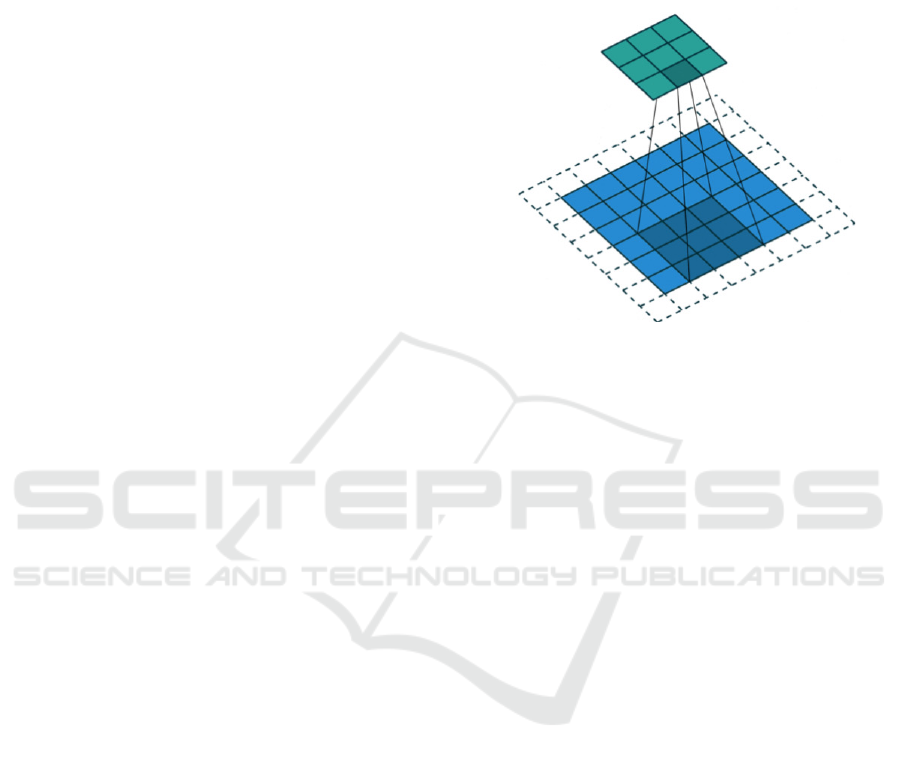
it’s like any other neural network. We’ll use a convo-

lutional neural networks (CNN) (Zhang et al., 2016),

which outputs a single number output for every im-

age. We’ll use stride of 2 to progressively reduce the

size of the output feature map (see Figure 5).

Figure 5: Filter hyperparameters.

Stride=2: For a convolutional or a pooling oper-

ation, the stride S denotes the number of pixels by

which the window moves after each operation.

Since the discriminator is a binary classiﬁcation

model, we can use the binary cross entropy loss func-

tion to quantify how well it is able to differentiate be-

tween real and generated images.

In this scenario, we use RMSprop optimizer

(Rome, 2017) which is similar to the gradient de-

scent algorithm with momentum. The RMSprop op-

timizer restricts the oscillations in the vertical direc-

tion. Therefore, we can increase our learning rate and

our algorithm could take larger steps in the horizontal

direction converging faster and forced to training the

GAN as follows:

1. Generation of a batch of images using the genera-

tor, it is passed through the discriminator.

2. Calculation of the loss by setting the target labels

to 1, in order to ”fool” the discriminator.

3. Use of the loss to perform a gradient descent, that

is to say to modify the weights of the generator,

so that it improves to generate realistic images to

”fool” the discriminator.

Now that after trained the models, we obtained

these results:

We can visualize how the loss changes over time.

Visualizing losses is quite useful for debugging the

training process. For GANs, we expect the genera-

tor’s loss to reduce over time, without the discrimina-

tor’s loss getting too high.

As can be seen in Figure 6, the loss at the level of

the discriminator stabilizes quickly around 0.6 while

ICEIS 2022 - 24th International Conference on Enterprise Information Systems

434

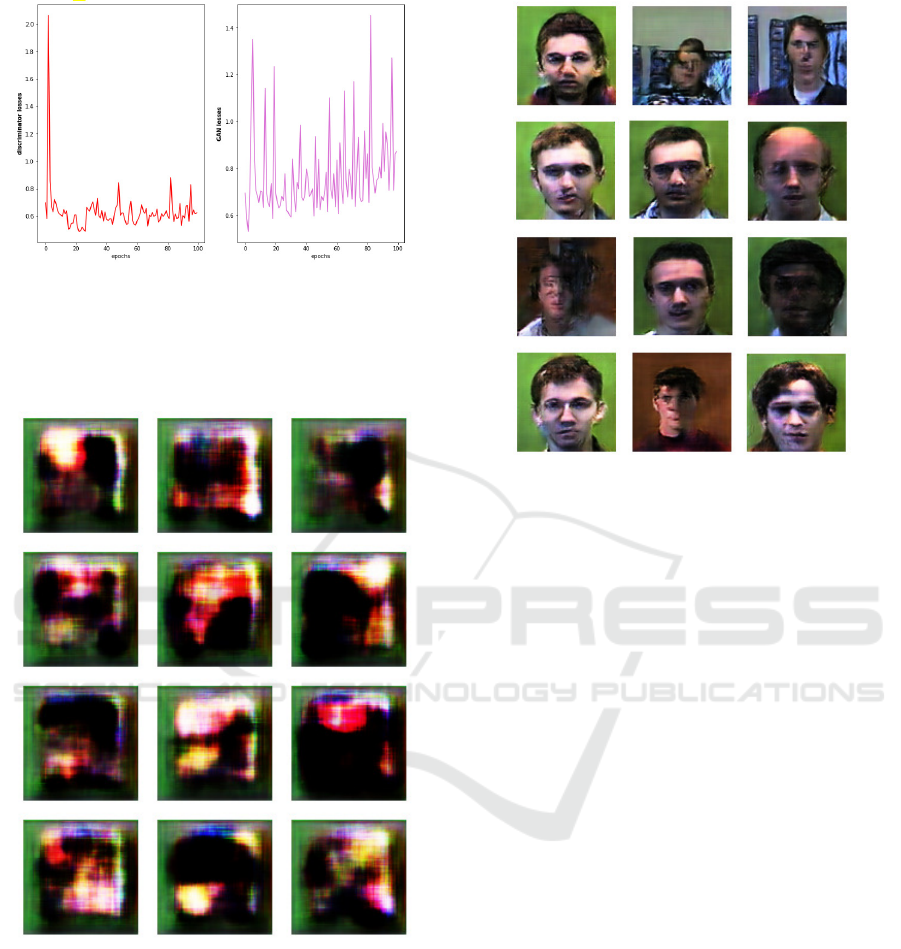
Figure 6: Left: Discriminator Loss. Right: Gan Loss.

that of the GAN (generator and discriminator) it os-

cillates around 0.8.

Well then this is what learning looks like so at the

beginning we start from noise:

Figure 7: First image generated.

So there (Figure 7) we don’t see it but it’s slightly

crude, and after a certain number of learning cycles

we see fairly quickly images that look like deformed

faces. But if they are not well drawn there is still

something that really looks like faces.

So let’s go here (Figure 8) we see that the faces

are more and more precise.

Figure 8: Image generated with more epochs.

4.8.2 Second Scenario

On this case, we add the encoder block portion and

using same padding so that the input and output di-

mensions are the same, as well as batch normalization

and leaky ReLU. Stride is mostly optional, as is the

magnitude for the leaky ReLU argument. Followed

by the discriminator itself in which we have recycled

the encoder block segment and are gradually increas-

ing the ﬁlter size to solve the problem we previously

discussed on ﬁrst scenario. We are performing the

opposite of the convolutional layers. The strides and

padding are the same for ease of implementation, and

we use batch normalization and leaky ReLU. On the

the generator side , we use decoder blocks and grad-

ually decrease the ﬁlter size. The choice of optimiza-

tion algorithm for a deep learning model can mean

the difference between good results in minutes, hours,

and days. The Adam optimization algorithm is an

extension to stochastic gradient descent that has re-

cently seen broader adoption for deep learning appli-

cations in computer vision and natural language pro-

cessing. So it is used in this second scenario to com-

pile disciminator.

We see that on this architecture (Figure 9) con-

sensus optimization achieves much better end results.

And the two losses converge to a relatively acceptable

value (0.2).

The images produced by the generator present a

relatively better quality than that of the ﬁrst scenario

(see Figure 10).

Impact of Hyperparameters on the Generative Adversarial Networks Behavior

435

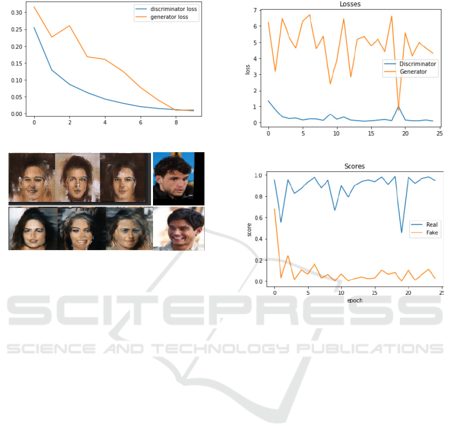
Figure 9: Discriminator & Generator Loss.

Figure 10: Image generated in 2nd scenario.

4.8.3 Third Scenario

This example is based on Minifaces dataset. We will

also scale and crop the images to 3x64x64, and nor-

malize the pixel values with a mean and standard de-

viation of 0.5 for each channel. This will ensure that

the pixel values are in the range (-1, 1), which is more

convenient for training the discriminator.

The input to the generator is typically a vector of

random numbers which is used as a seed to generate

an image. The generator will convert a latent shape

tensor (128, 1, 1) into a 3 x 28 x 28 shape image ten-

sor. The adjustment function to train the discriminator

and the generator in tandem for each batch of training

data uses the Adam optimizer. We will also save sam-

ple generated images at regular intervals for inspec-

tion.

The ﬁgures 11 and 12 show ﬂuctuations in the

scores and errors of the generator, which explains the

variation in image quality from one epoch to another

(See Figure 13).

In table 1 the average of the error of the genera-

tor for dataset Minifaces is too high with an exces-

sive ﬂuctuation. As a result, some images appear rel-

atively distorted.

4.8.4 Forth Scenario

In this example we describe a GAN witch, when

trained is able to generate samples indiscernible from

those sampled from the normal distribution (ﬁgure

Figure 11: Discriminator & Generator Loss.

Figure 12: Discriminator & Generator Score.

14). The standard normal distribution (ﬁgure14), also

called the z-distribution, is a special normal distribu-

tion where the mean is 0 and the standard deviation is

Figure 15 illustrates the learning to sample from

the standard normal distribution. The network con-

tains one hidden layer of 16 ReLU units on the gen-

erator and 64 on the discriminator. The function rep-

resented in ﬁgure 14, also called the z-distribution, is

a special normal distribution where the mean is 0 and

the standard deviation is 1.

After the training the gan for about 600 epochs we

obtained the results (Figure 15).

For the three examples below, In the process of

learning the discriminator network, it is fundamental

to label the real images as ”true” and the false images

as ”false”. However, after a while of training, the sys-

tem will be stimulated by the use of deceptive strate-

gies that ”surprise” the discriminator. and constrain it

to make corrections to what had already been learned

before. These strategies consist of labeling the gener-

ated images as if they were ”real”. This technique al-

lows the generator to make the necessary corrections

and thus prove to be faces more resembling those pro-

vided as a model.

ICEIS 2022 - 24th International Conference on Enterprise Information Systems

436

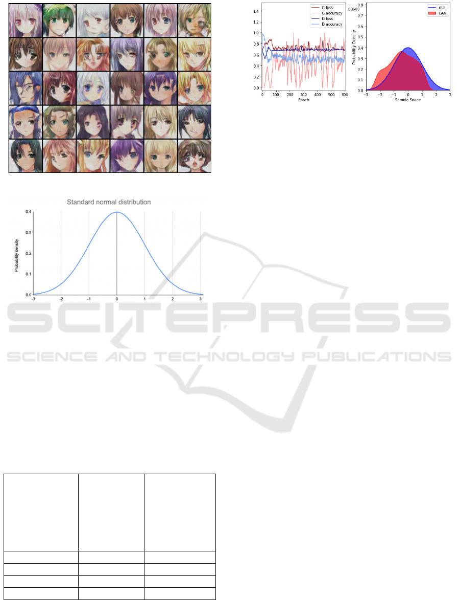
Figure 13: Images generated in scenario 3.

Figure 14: standard normal distribution.

The same deceptive strategy is adopted for the

last example, which forces the descimnator to pro-

duce curves resembling the model provided as input

(Figure15). After 600 epochs the generated curve

tends towards a distribution curve with some defor-

mations (Figure15 Right)

The performance of the GAN depends on the data

processed. The models are large and complex and

take a lot of communication and memory and require

some real computational horsepower.

Table 1: Hyper-parameters optimization and losses.

Scenario

Discriminator Loss

Generator/GAN Loss

1-Faces 0.6 0.8

2-Celeb 0.2 0.2

3-Minifaces 0.2 4.5

4 z-distribution 0.7 0.7

Figure 15: A GAN learning to sample from the standard

normal distribution over 600 epochs.(Left) the accuracies

and losses of the generator and discriminator (Right) the

observed probability density of the GAN and the real N(0,

1) density.

5 CONCLUSIONS

Generative adversarial networks models are not able

to formulate an intention and assess their own results

and therefore are not completely autonomous creative

systems. The dataset on which the GAN is trained is

the key to its creativity. GAN is a powerful structure

that stimulates feature extraction but is unstable with

its convergence uncertainty during training. Its con-

tradictory insight is the main motivation improvement

of the model but its structure is too simple and has

many unknowns factors affecting its results which ex-

plains its instability. We propose a relatively stable set

of architectures for the training of generative adver-

sarial networks and we provide evidence that adver-

sarial networks learn good image representations for

supervised learning and generative modeling. How-

ever there are still some forms of model instability.

In order to resolve this instability issue, further

work is required. We believe that the broader func-

tional coverage encompassing other areas such as

video and speech (pre-trained features for speech syn-

thesis) should be very interesting. Also, how the acti-

vations performed on large-scale data still need to be

investigated.

Further research on the properties of learned latent

space would also be interesting.

REFERENCES

(2015). Unsupervised Representation Learning with

Deep Convolutional Generative Adversarial Net-

works. OCLC: 1106228480.

Abdollahpouri, H., Adomavicius, G., Burke, R., Guy, I.,

Jannach, D., Kamishima, T., Krasnodebski, J., Piz-

zato, L., and SpringerLink (Online service) (2020).

Multistakeholder recommendation: Survey and re-

search directions. OCLC: 1196494457.

Impact of Hyperparameters on the Generative Adversarial Networks Behavior

437

Alec, R., Metz, L., and Chintala, S. (2015). Unsuper-

vised Representation Learning with Deep Convolu-

tional Generative Adversarial Networks. OCLC:

1106228480.

Barua S, Erfani S.M, and Bailey J (2019). FCC-GAN: A

fully connected and convolutional net architecture for

GANs. arXiv arXiv. OCLC: 8660853988.

Brophy, E., De Vos, M., Boylan, G., and Ward, T. (2021).

Multivariate Generative Adversarial Networks and

Their Loss Functions for Synthesis of Multichannel

ECGs. IEEE Access IEEE Access, 9:158936–158945.

OCLC: 9343652742.

Brownlee, J. (2020). How to Code the GAN Training Algo-

rithm and Loss Functions.

Denton, E., Chintala, S., Szlam, A., and Fergus, R.

(2015). Deep Generative Image Models using a

Laplacian Pyramid of Adversarial Networks. OCLC:

1106220075.

Goodfellow, I. (2016). NIPS 2016 Tutorial: Generative Ad-

versarial Networks. OCLC: 1106254327.

Goodfellow, I. J., Pouget-Abadie, J. P., Mirza, M., Xu, B.,

Warde-Farley, D., Ozair, S., Aaron, C., and Bengio,

Y. (2020). Generative adversarial networks. Commun

ACM Communications of the ACM, 63(11):139–144.

OCLC: 8694362134.

Jarrett, K., Kavukcuoglu, K., Ranzato, M., LeCun, Y., and

2009 IEEE 12th International Conference on Com-

puter Vision (ICCV) (2009). What is the best multi-

stage architecture for object recognition? pages 2146–

2153. OCLC: 8558012250.

Jessica, L. CelebFaces Attributes (CelebA) Dataset.

Jiang, Y., Gong, X., Ding, L., and Yu, C. (2019). Enlight-

enGAN: Deep Light Enhancement without Paired Su-

pervision. OCLC: 1106348980.

Mao, X. and Li, Q. (2021). Generative Adversarial Net-

works for Image Generation. OCLC: 1253561305.

Mayer, C. and Timofte, R. (2020). Adversarial Sampling

for Active Learning. In 2020 IEEE Winter Conference

on Applications of Computer Vision (WACV), pages

3060–3068, Snowmass Village, CO, USA. IEEE.

Parthasarathy, D., Backstrom, K., Henriksson, J., Einars-

dottir, S., and 2020 IEEE International Conference On

Artiﬁcial Intelligence Testing (AITest) (2020). Con-

trolled time series generation for automotive software-

in-the-loop testing using GANs. pages 39–46. OCLC:

8658758958.

Rocca, J. (2021). Understanding Generative Adversarial

Networks (GANs).

Rome, S. (2017). An Annotated Proof of Generative Ad-

versarial Networks with Implementation Notes.

Sandy, E., Ilkay, O., Dajiang, Z., Yixuan, Y., and Anirban,

M. Deep Generative Models, and Data Augmenta-

tion, Labelling, and Imperfections : First Workshop,

DGM4MICCAI 2021, and First Workshop, DALI

2021, Held in Conjunction with MICCAI 2021, Stras-

bourg, France, October 1, 2021, Proceedings (Livre

num

erique, 2021) [WorldCat.org].

Stewart, M. Introduction to Turing Learning and GANs |

by Matthew Stewart, PhD Researcher | Towards Data

Science.

Sun H, Deng Z, Parkes D.C, and Chen H (2020). Decision-

aware conditional GANs for time series data. arXiv

arXiv. OCLC: 8694375343.

Tae, J. (2020). The Math Behind GANs.

Tanaka, M., Shibata, T., Okutomi, M., and 2019 IEEE Inter-

national Conference on Consumer Electronics (ICCE)

(2019). Gradient-Based Low-Light Image Enhance-

ment. pages 1–2. OCLC: 8019257222.

Zhang, X.-J., Lu, Y.-F., Zhang, S.-H., and SpringerLink

(Online service) (2016). Multi-Task Learning for Food

Identiﬁcation and Analysis with Deep Convolutional

Neural Networks. OCLC: 1185947516.

Zhu, J.-Y., T, P., P, I., and Efros A.A (2017). Unpaired

image-to-image translation using cycle-consistent ad-

versarial networks. arXiv arXiv. OCLC: 8632227009.

ICEIS 2022 - 24th International Conference on Enterprise Information Systems

438