Using the Silhouette Coefficient for Representative Search of

Team Tactics in Noisy Data

Friedemann Schwenkreis

Baden-Wuerttemberg Cooperative State University, Paulinenstr. 50, 70565 Stuttgart, Germany

Keywords: Data Science, Clustering, Team Handball, Tactics Recognition.

Abstract: Automatically recognizing team tactics based on spatiotemporal data is challenging. Deep Learning

approaches have been proposed in this area but require a tremendous amount of manual work to create training

and test data. This paper presents a clustering approach to reduce the needed manual effort significantly. A

method is described to transform the spatiotemporal data into a canonical form that allows to efficiently apply

clustering techniques. Since noise cannot be avoided in the given application context, the silhouette coefficient

is applied to filter clusters considered to be noisy in a cluster technique independent way. Then, a variant of

the silhouette coefficient is introduced as an indicator regarding the overall cluster model quality which allows

to select the optimal clustering technique as well as the optimal set of cluster technique parameters for the

given application context.

1 INTRODUCTION

The application area of team tactics recognition in

team sports uses the players’ positions and data

mining methods to automatically detect reoccurring

tactical moves of teams. It has been proposed to use

deep-learning-based classification techniques like

(T)CNNs to solve this task (Schwenkreis, 2018a).

However, the challenge of classification approaches

is to find enough training and test data to extract a

model with sufficient quality.

In the field of team sports like team handball, this

means, that large sets of position data need to be

manually labelled by experts before the actual model

extraction can be performed. Particularly in case of

deep learning models, this results in a tremendous

amount of manual effort and requires a lot of time,

because the experts need to watch videos that

correspond with the positional data in order to be able

to classify a move that happens in a given interval.

This paper presents an approach to reduce the

manual effort significantly. The concept of

representative search based on clustering is used to

identify representatives of a group of similar team

moves. When a representative is manually classified,

then it is assumed that a whole cluster of similar team

https://orcid.org/0000-0003-4072-0582

moves belongs to the same class. Thus, not each team

move needs to be classified manually to get the

training and test data but only one per group.

Alternatively, the labelled clustering model can be

used directly to “classify” new data.

The results presented in this paper have been

derived from data of five handball games from which

272 situations have been extracted that potentially

contain a team tactic. Section 2 describes the method

to transform the available data such that clustering

methods can be applied. Section 3 introduces the

notion of similarity that is used in case of team tactics.

In section 4 the approaches of handling noise and

selecting an appropriate clustering method are

presented. Section 5 concludes the paper with a

summary of the results and an outlook on future work.

2 CANONICAL POSITIONAL

DATA

The starting point of the analysis presented in this

paper is data from team handball matches. To be more

specific, it is data of matches of the first German

handball league (HBL), collected using the player

tracking system of Kinexon® (Kinexon, 2017). This

Schwenkreis, F.

Using the Silhouette Coefﬁcient for Representative Search of Team Tactics in Noisy Data.

DOI: 10.5220/0011100600003269

In Proceedings of the 11th International Conference on Data Science, Technology and Applications (DATA 2022), pages 193-202

ISBN: 978-989-758-583-8; ISSN: 2184-285X

193

means that the data consists of the 3D coordinates of

the sensors carried by the players between the

shoulders, as well as of the coordinates of a sensor

built into the ball. Since the elevation is not of interest

in the context of the presented work, the data is

reduced to 2D coordinates ranging roughly from (0,0)

to (40,20), which are the dimensions of a team

handball field in meters.

The positional data is generated every 50 ms by

the Kinexon system and each component of the

coordinates is provided with an accuracy of three

digits after the decimal separator. However, the actual

spatial accuracy of the Kinexon system is lower and

the location of a player might be given with an overall

accuracy of about 10 cm. Thus, the data has been

reduced to a single digit after the decimal separator.

2.1 Basic Definitions

A team positional state (tpos) at a certain point in time

is an ordered set of up to seven player coordinates,

depending on the number of players who are currently

allowed on the field (there might be suspended

players which reduces the number of players on the

field) plus the coordinates of the ball. The match

positional state (mpos) at a given point in time is the

union of the two team positional states (the ball

coordinates are contained only once in the mpos).

A team tactical move (ttm) can then be defined as

an ordered set of team positional states of the same

team during a certain timeframe contained in a match.

Based on observations of real-world data, it has been

decided to use 5.5 seconds as the timeframe for a team

tactical move. Given the Kinexon rate of 20 pairs of

coordinates per second, a team tactical move is

represented by 880 pairs of coordinates in the data.

Finally, we can define an individual positional

state as the coordinates of a player or the ball at a

specific point in time and a trajectory of a ttm as the

extract of all individual positional states of a single

player or the ball from a team tactical move in the

temporal order of the contained coordinates.

2.2 Challenges of Data Preparation

There are four basic challenges to get comparable

data of team tactical moves collected from team

handball matches:

 To be able to compare the coordinate values of

ttms, the start and end of a ttm needs to be

determinable and deterministic.

 There is no fixed schema for the origin of the

coordinates of different matches. The origin

depends on the location of the table of the

timekeeper of a match. The left lower corner

from the timekeeper’s perspective has always

the coordinates (0,0).

 Team tactics in team handball are mostly

restricted to the half of the field with the goal

against which an attack happens. However, this

part of the field changes with every attack.

Thus, there are attacks in which most x-

coordinates are significantly below 20m and

there are attacks with most x-coordinates

significantly above 20m.

 Sides are switched after half time break. This

results in a change of attack coordinates from a

player’s perspective: If the same player has for

instance attack coordinates in the range of (0,0)

to (4, 5) in one half, a typical left-wing player,

the same player has attack coordinates in the

range of (36, 15) to (40,20) in the second half.

 The order of the players’ coordinates of a team

tactical move is arbitrary.

In the following the approaches to overcome these

challenges are presented.

2.3 Timeframes of Team Tactical

Moves

Particularly, the first challenge presented in the

previous section, to have well-defined points in time

when team tactical moves start and end, requires

using knowledge beyond the positional data. For that

purpose, additional match data is used (Schwenkreis,

2018b).

Since a ttm is only of interest in the context of this

work if an attempt to score is made, the timeframe of

a ttm is defined as follows:

 The end of a team tactical move is defined as

the last tpos in which the ball is closest to the

attempting player before the recorded

timestamp of the attempt.

 The start of a team tactical move is 109 tposs

before the last tpos. Thus, a team tactical move

consists of 110 tposs.

2.4 Transformation of Coordinates

The second, third and fourth challenges described in

section 2.2 denote the problem of “changing”

coordinate values. Even if the “tactical” position of a

player is the same with respect to his or her team, the

values of his/her coordinates can be different. Thus, a

concept is needed to avoid the changing origins and

changing playing directions.

DATA 2022 - 11th International Conference on Data Science, Technology and Applications

194

Again, the additional match data in combination

with handball specific knowledge help to transform

the data into a canonical format. Team tactics in team

handball are used to generate situations in which an

attempt has a high scoring probability. If the opponent

team is playing with a goalkeeper, then the high

scoring probability will only be achieved, if the

attempting player is in the same half of the field as the

opponent’s goal. There are cases in which the

attempting player is not in the half of the opponent’s

goal, but these cases are irrelevant for team tactics

because in these cases the opponent’s goalkeeper is

usually not present (or just about to return to the goal)

and thus no explicit tactics are applied.

Based on this observation, we can state that in

case of the relevant cases in the context of this work,

the attempting player needs to have a x-coordinate

between 0 and 20, given that the opponent’s goal has

a x-coordinate of 20. If the x-coordinate of the

attempting player is above 20, then we assume that

we need to transform the coordinates of all players

and the ball. I.e., we need a point reflection of the

coordinates using the centre of the field.

As a result, all coordinates are transformed such

that there are only attempts against the goal “of the

right side of field” (from the point of view of the

timekeeper of a match). Thus, the previously

described challenges two to four of section 2.2 are

resolved.

2.5 Sort Order of Player Coordinates

The concept of representing ttms as vectors has been

introduced previously (Schwenkreis, 2018a). In this

previous work, it has been proposed to use

classification based on deep learning. To overcome

the problem of “non-deterministic” ttm vectors, all

permutations of players of the ttm representing vector

were used to train the deep learning model. Now, if

clustering is used rather than classification, it does not

make sense to generate all permutations because it

would significantly distort the clustering result. It is

rather necessary to generate an order of players that is

well-defined.

From the point of view of team tactics there is no

need for a sort order across teams. It is rather

sufficient to have a well-defined sort order for each

team. Furthermore, it is irrelevant which sort order is

chosen as long as the sorting results in the same

sequence of player coordinates for all ttms that are to

be compared. Furthermore, it is important to ensure

that the vector position of a specific player remains

the same across all tposs of a ttm.

To determine the vector position of a player in

tposs, a heuristic is used that is derived from the

handball method to number the players by their

assigned offense position on the field: The “left-

wing” player is numbered one, the “half-left” player

two and so on. Finally, the goalkeeper gets number 7

and the ball number 8.

The offense position of players is defined by the

line-up data which is part of the additional match data

mentioned in section 2.3. For example, the player

who has been assigned to the “left-wing” position in

the line-up is assigned the vector position one as his

or her “coordinate index” in a tpos.

Some special cases need to be considered with

this approach: There might be the case when two

players with the same “nominal” offense position are

on the field, which would result in the same

coordinate index and an empty pair of coordinates in

the tpos. In this case, the y-coordinate in the starting

position of the tpos is used to determine the

coordinate index. There are three groups that are

handled separately: The two players with positions on

the left side, the three players in the mid and the two

players with positions of the right side.

 In case of the offensive team, the player with

the highest y-coordinate is treated as the player

with the position defined in the line-up record.

Then the next empty coordinate slot in the same

player group of the tpos with a higher index is

used for the second highest y-coordinate.

 In case of the defending team, the player with

the lowest y-coordinate is treated as the player

with the position defined in the line-up record.

The next empty coordinate slot in the player

group of the tpos with a lower index is used for

the player with the second lowest y-coordinate.

 Cases with more than two players with the

same assigned position in the line-up are not

covered at this point.

3 TEAM MOVEMENT

SMIILARITY

Like classification clustering belongs to the family of

segmentation methods. The basic difference between

the two approaches is that clustering needs an explicit

notion of similarity (or distance), while classification

derives this notion implicitly based on the attribute

values of records with the same class label. Since the

assignment of class labels is very costly in the given

application scenario, the use of a non-supervised

approach based on clustering is proposed. Thus, a

Using the Silhouette Coefﬁcient for Representative Search of Team Tactics in Noisy Data

195

suitable notion of similarity needs to be selected or

defined respectively.

Clustering to find groups of similar tactics means

to find groups of similar ttms. Hence, we need to

define a notion of similarity for ttms. However, a ttm

consists of the discretized trajectories of involved

players and the ball. Thus, the similarity of two ttms

depends on the similarity of the contained individual

projections of the ttms.

3.1 Distance of Trajectories

Since the trajectories described by the individual

projections of a ttm consist of the spatiotemporal data

of the players and thus of an ordered sequence of 2D-

coordinates, it makes sense to define the similarity of

two trajectories based on a distance criterion. It is

easy to calculate the Euclidean Distance of the 110

points that are part of an individual projection of a

ttm, but there are multiple options for the aggregated

distance of the two (Kumar, Chhabra, & Kumar,

2014).

Given the total order of the points of the

trajectories based on the timestamps of the

coordinates and the fact that all trajectories consist of

the same number of points, the Discrete Fréchet

Distance D has been selected as the aggregated

distance of two trajectories (Aronov, Har-Peled,

Knauer, Wang, & Wenk, 2006). Given two

trajectories A and B of the same time interval T, D is

the maximum Euclidean Distance d of any two points

(t) and p

(t) contained in A and B at any given point

in time t of the interval T.

𝐷(

𝐴

,𝐵)=max

∀



∈



𝑑(𝑝



(

𝑡

)

,𝑝



(

𝑡

)



(1)

3.2 Distance of Two Sets of

Trajectories

To define the distance of two ttms, we need to

aggregate the distances of the trajectory pairs of each

contained player (and the ball). Again, there are

multiple options to aggregate these trajectory

distances and the process of identifying the optimal

aggregation function is still ongoing.

The challenge is to find an aggregation function

that matches the human perception of the similarity

of team tactical moves. There are at least some

application specific details which help to narrow

down the degree of freedom:

 Goalkeepers are usually not involved in team

tactics. In fact, there are only very few tactics

that involve more than 4 players.

 Having some close trajectories compensates

for far trajectories to some extent.

 The ball can only be part of a team tactical

move in case of the offensive team – the

defensive team does not have the ball.

 The ball moves much faster than the players

which also leads to larger differences of the

trajectories. In average, the differences of ball

trajectories are three times the differences of

the player trajectories. Hence, the trajectory

distances of the ball are multiplied with a factor

of one third to compensate for the differences

in velocity.

Overall, the distance value ΔT of two ttms, A and

B, is defined as the mean value of the trajectory

distances of the contained players A

to A

and B

respectively (see section 2.5). In case of the

offensive team, the distance of trajectories of the ball

and B

) might be added to the calculation of the

mean value.

∆𝑇

.

𝐷

(

𝐴



,𝐵



)

+𝐷

(

𝐴



,𝐵



)









(2)

∆𝑇=

𝐷

(

𝐴



,𝐵



)









(3)

4 CLUSTERING ASPECTS

4.1 Constraints

Clustering denotes the search for groups of similar

data sets and there are quite several different

approaches to it (Xu & Tian, 2015). In the given

application context, we have constraints which limit

the applicability of some approaches.

The given trajectories might represent a team

tactical move, but they also might not contain a move

that qualifies as a real tactical move. Some attacks in

handball are finished based on individual decisions

rather than containing the coordinated move of

several players. Thus, the ttms containing an

individual move rather than a tactical move are

considered as noise in the context of clustering: They

should not be assigned to any cluster.

Furthermore, the number of played tactics is

unknown and there might be more tactics than

represented by the data set we are looking at. I.e., if

we need to specify the number of clusters upfront,

then we might have not enough clusters compared to

the number of tactics contained in our data set. As a

DATA 2022 - 11th International Conference on Data Science, Technology and Applications

196

result, some ttms might be treated as noise or they will

be assigned to clusters which consist of records that

are not similar from a handball perspective.

On the other hand, there is the case when we

specify too many clusters. In that case we want the

clustering approach to allow empty clusters rather

than enforcing the assignment of at least one record

to each cluster.

4.2 Considered Methods

Given the constraints of section 4.1, all clustering

methods have been excluded hat require to specify the

number of clusters upfront unless empty clusters are

supported. The following three methods have been

evaluated in the described context

4.2.1 DBSCAN

A method fulfilling all described constraints is

Density-Based Spatial Clustering of Applications

with Noise or short DBSCAN (Ester, Kriegel, Sander,

& Xu, 1996). The method searches for clusters based

on the criterion that there is a certain minimum

number of close neighbours of a data point (also

denoted as node). Further points are added to the

cluster if they are direct close neighbours, or in case

they are indirect close neighbours of other

neighbouring nodes. If points do not have the

minimum number of neighbours, they are treated as

noise, i.e., they are assigned to a special noise cluster.

Two parameters of the method influence the result

of DBSCAN significantly:

 The distance that is used to identify direct

neighbours.

 The minimum number of neighbours that is

needed to build a cluster.

Given the two parameters, DBSCAN finds an

arbitrary number of clusters of arbitrary shape.

4.2.2 Hierarchical Clustering

Both, Divisive Hierarchical Clustering as well as

Agglomerative Hierarchical Clustering do not require

to specify the number of clusters upfront. They both

generate a hierarchy with the points of the data set at

the leaves based on the application specific distances

between the points (Murtagh & Contreras, 2012).

Then the tree representing the hierarchy can be

interpreted as a set of clusters by evaluating the links

of a certain level in the tree.

In the context of this work, the evaluation of the

links is done using the inconsistency coefficient as a

criterion (Martinez & Martinez, 2005). The

inconsistency coefficient can be calculated for each

link in the tree, which are potential clusters. When a

link has an inconsistency coefficient that is lower than

a specified maximum inconsistency coefficient, it is

accepted as a cluster. Child links of the identified link

in the hierarchy are not further evaluated.

With this approach there might be clusters

consisting of single points of the data set, because the

leave level has an inconsistency coefficient of 0 and

thus qualifies in case no parent link has qualified

before. These clusters are treated as noise. In the

context of this paper only the agglomerative variant

of hierarchical clustering is further evaluated.

4.2.3 Self-Organizing Maps

Self-Organizing Maps (SOMs) or Kohonen Networks

belong to the family of artificial neural networks (van

Hulle, 2012). They require the specification of the

length and width of a rectangular shaped two-

dimensional output area of neurons. The length and

width are expressed as the number of neurons of each

dimension and the product of the two corresponds to

the maximum number of clusters that can be

distinguished. SOMs “tolerate” empty clusters in the

sense that it does not negatively impact the model

when no input record is depicted on a certain output

neuron.

SOMs are very flexible in terms of the cluster

shapes which can be identified but they do not take

into account the notion of an application specific

distance. On the other hand, they have several

parameters that allow to adjust the SOMs for specific

needs as:

 The number of output neurons in each

dimension.

 The size of the neighbourhood of a neuron.

 The layer topology function.

 The distance function to calculate the distance

between the weights of neurons and input sets.

As in case of hierarchical clustering, SOMs might

generate clusters consisting of single records. To be

specific, the clustering model depicts just a single

record on a certain output neuron when the trained

network is applied to the training set. These “single”

records are treated as noise.

4.3 Cluster Model Quality

4.3.1 Basic Criterion

A very important aspect of clustering is the evaluation

of the extracted clustering model. Particularly when

comparing clustering methods or parameter settings

Using the Silhouette Coefﬁcient for Representative Search of Team Tactics in Noisy Data

197

of clustering methods, a metric is needed that allows

to rank the approaches and settings thereof.

There is a multitude of so-called validity indexes

for clustering (Saitta, Raphael, & Smith, 2008). In the

scope of this work, we selected the silhouette

coefficient as the base criterion for the following

reasons:

 It is calculated based on the application specific

notion of distance.

 The computational complexity is low if

distances of the records of the dataset can be

pre-calculated – which is possible in our case.

 It takes into account the cluster density as well

as the distance to other clusters. The silhouette

coefficient ranges between -1 and +1 and

values below 0 are indicating a bad cluster

association of a record.

 It can be calculated for each point of the data

set, for a cluster and for an overall cluster

model. The silhouette coefficient of a cluster is

the mean value of the silhouette coefficients of

the contained records. The silhouette

coefficient of a model is the mean value of all

records.

Furthermore, the visualization of silhouette

coefficients as a silhouette plot provides a simple

means for the intuitive evaluation of a clustering

model (MathWorks, 2022).

However, there are drawbacks that come with the

silhouette coefficient. Since the aggregation of the

silhouette values of clusters is done based on

calculating the average of the silhouette coefficients

of the contained records, the silhouette coefficient is

well suited for clusters with a convex shape but has

limitations in case of concavely shaped clusters.

Furthermore, having a model consisting of a single

cluster, results in a silhouette coefficient of 1 which

indicates a perfect clustering model.

When data is present that has been identified as

noise, the calculation of the silhouette coefficient

needs to be adjusted accordingly. Noise should not

influence the values of the silhouette coefficients.

Thus, special noise clusters and contained data must

be excluded before the calculation of the silhouette

coefficients.

4.3.2 Weighted Silhouette Coefficient

There are multiple extreme cases when varying the

parameters of clustering models:

 All records are treated as noise and no cluster

is identified. The silhouette coefficient is not

defined in this case.

 Only a single cluster with a low number of

records is identified, while all other records are

treated as noise. Then, the silhouette coefficient

reaches its maximum.

 All non-noise records are part of a single

cluster. This is like the sphere surrounding all

data points Again, the silhouette coefficient

becomes maximal in this case.

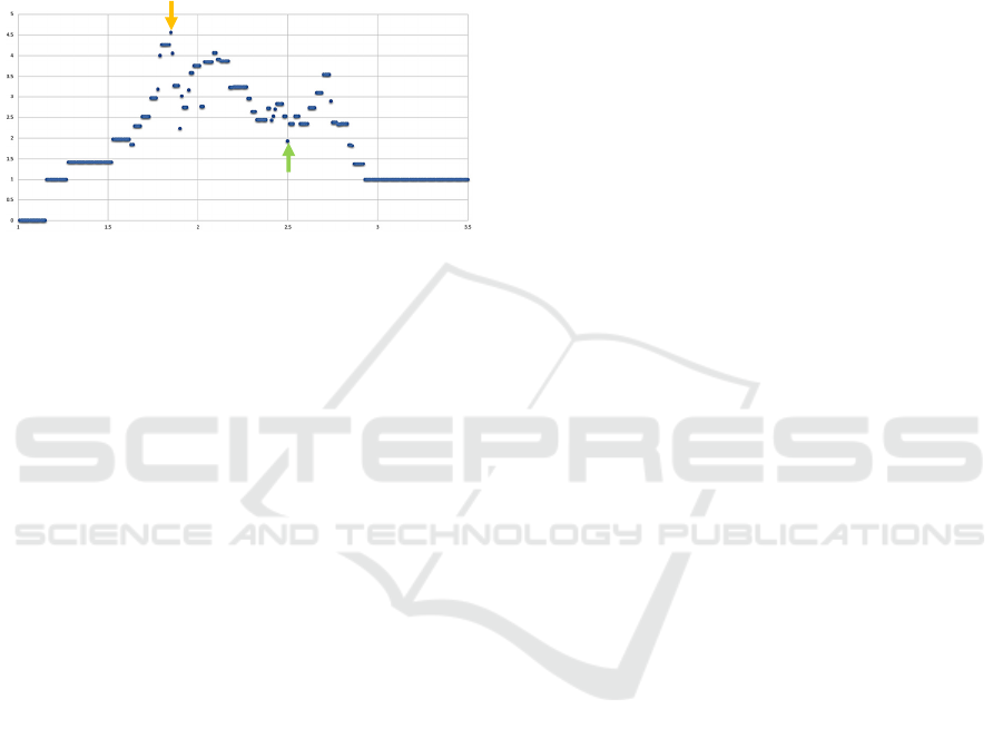
Particularly in case of the DBSCAN clustering

method, all three cases can be created easily when

varying the minimum distance parameter for

identifying neighbours. As depicted in Figure 1, there

is only noise until a value of approximately 1.3 and

no silhouette coefficient value is depicted. Then the

first cluster is identified, and the silhouette coefficient

becomes 1. With increasing values of the minimum

distance, the value of the silhouette coefficient varies

until around a minimum distance of 3. Then all

records are considered to belong to the same cluster

and the silhouette coefficient jumps back to 1.

Figure 1: Distribution of DBSCAN silhouette coefficient

values over a variation of the minimum distance parameter,

defence data.

When looking for the optimal distance to be used

with the DBSCAN method, the direct interpretation

of the silhouette coefficient does not help. In the case

depicted in Figure 1, the local maximum around 2.5

seems to be the optimal point (indicated by the green

arrow), but there is no general rule that allows to

determine it.

Therefore, knowledge of the application level has

been used to find an appropriated indicator. When

searching for team tactics in terms of similar ttms, we

need to compromise between a clustering model with

an optimal silhouette coefficient and the number of

clusters that are detected. It is known upfront that

there must be more than one cluster. In fact, we know

for sure that there are more than 10 clusters.

Thus, we use a weighted silhouette coefficient ws

as the validity index of a clustering model M. The

weighted silhouette coefficient is defined as the

product of the silhouette coefficient s(M) of a

DATA 2022 - 11th International Conference on Data Science, Technology and Applications

198

clustering model and the number of identified clusters

c contained in M:

𝑤𝑠

(

𝑀

)

=𝑠

(

𝑀

)



𝑐





,𝑐



∈𝑀

(4)

An alternative weighting with the number of

records that are contained in the set of identified

clusters has been discarded, because it also becomes

maximal when all records are grouped into a single

cluster.

Figure 2: Distribution of the weighted DBSCAN silhouette

coefficient values over a variation of the minimum distance

parameter, defence data.

Figure 2 shows the distribution of the weighted

silhouette coefficient given the same variation of the

minimum distance parameter as depicted in Figure 1.

The global maximum value of ws

is reached at a

minimum distance of 1.85 (indicated by the orange

arrow) which is significantly different from the

minimum distance of the local maximum of the non-

weighted silhouette coefficient value: 2.5 (green

arrow in Figure 2). It is surprising that the non-

weighted silhouette coefficient has a local minimum

at 1.85 (orange arrow in Figure 1) while the weighted

silhouette coefficient has a maximum and that the

weighted silhouette coefficient has a local minimum

at 2.5 while the silhouette coefficient has a maximum.

We do not have an explanation for this phenomenon

at this point.

4.3.3 Advanced Handling of Noise

As mentioned in section 4.2, not all considered

clustering techniques have an explicit notion of noise.

Even worse, the SOM method cannot even apply the

application specific distance function to identify

noise. Nevertheless, it must be ensured, that noise

does not impact the clustering model, whether the

technique that generated the model considers an

application specific distance function or not.

It has already been described in section 4.2 that

clusters consisting of a single record are treated as

noise although they have a silhouette coefficient of 1.

Furthermore, the application area is only interested in

having records being assigned to a cluster if there is a

minimum certainty that the record belongs to the

cluster. As mentioned in the introduction, we are

looking for representatives and each record of a

cluster should be a valid representative for a whole

cluster. Hence, a minimum silhouette coefficient is

required for all records. Records with a silhouette

coefficient less than the minimum record-level

silhouette coefficient are treated as noise as well. The

results presented in this paper have been calculated

using a record-level minimum silhouette coefficient

of 0.1.

In addition to the record-level minimum

silhouette coefficient there is also a minimum cluster-

level silhouette coefficient which must be greater than

the minimum record-level silhouette coefficient to

have an effect. If a cluster has a silhouette coefficient

less than the minimum cluster-level silhouette value,

then all records of the cluster are treated as noise. A

cluster-level minimum silhouette coefficient of 0.3

has been used in the context of this paper.

Overall, the following “filtering” steps are applied

after the computation of a clustering model to derive

the final clustering model and to calculate the overall

silhouette coefficient:

 Records not having neighbours in the same

cluster are removed (including the clusters).

 Silhouette coefficients are calculated.

 Records with a low silhouette coefficient are

removed (see above) and records not having

neighbours in the same cluster are removed.

 Silhouette coefficients are recalculated.

 Clusters with a low silhouette coefficient and

contained records are removed (see above).

 Silhouette coefficients are recalculated, and the

overall ws of the model is calculated.

4.4 Comparing Clustering Methods

Since offense ttms and defence ttms differ

significantly, it cannot be assumed that the same

clustering method is optimal in both cases. Hence, the

method selection needs to be done two times, for the

offense case and the defence case.

The selection of the clustering technique to

generate the model for the representative search has

been a two-phased process:

 In phase 1 the optimal parameter setting for

each considered method was searched

 In phase 2 the previously found optimal

parameter settings were used to select the

optimal clustering technique.

In both phases the weighted silhouette coefficient is

used as the decisive factor.

Using the Silhouette Coefﬁcient for Representative Search of Team Tactics in Noisy Data

199

4.4.1 Investigated Parameter Settings

DBSCAN Parameters

In case of the DBSCAN method there are two major

parameters: The minimum distance of neighbour

points and the minimum number of points required to

build a cluster. The latter parameter was set to two

because it was assumed that some ttms were only

contained two times in the data given the available

amount of data (see introduction). Hence, only

variations of the minimum distance had to be

evaluated.

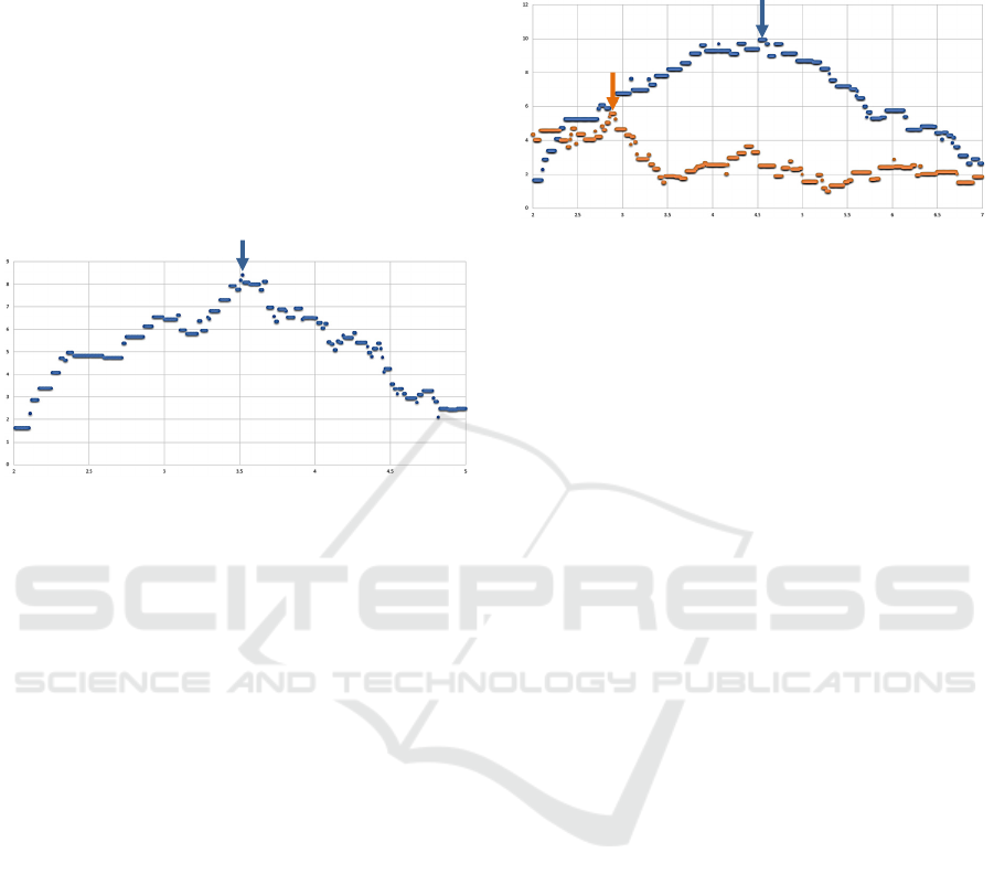
Figure 3: DBSCAN: weighted silhouette coefficient,

offense data.

To get an idea of the needed variations, the

minimum, and the maximum distances of all

available ttms have been calculated. It turned out that

the defence ttms have a closer distance than the

offense ttms and that we reach the maximum

weighted silhouette coefficient relatively early. In the

end it was sufficient to cover the range of [1,3.5] in

case of the defence ttms and the range of [2,5] in case

of the offense ttms. The resulting weighted silhouette

coefficient in the defence case has been depicted in

Figure 2. Figure 3 shows the corresponding values of

the offense case.

Hierarchical Clustering Parameters

The agglomerative hierarchical clustering itself does

not have any parameters and generates a complete

tree which is based on the application specific

distance function. The complete link criterion has

been used to generate the trees described in this paper.

On the other hand, the interpretation of the tree as a

clustering model is somewhat arbitrary. The approach

described in this paper uses the MATLAB™

inconsistency coefficient to determine the links in the

tree that are considered to be clusters of the clustering

model (Martinez & Martinez, 2005).

The inconsistency coefficient is a means for the

dissimilarity of the records belonging to a link. The

lower the value, the more similar are the records that

are connected to the link. From that perspective, the

inconsistency coefficient is similar to the minimum

distance parameter of the DBSCAN method.

Figure 4: Hierarchical Clustering: weighted silhouette

coefficients for offense (blue) and defence (orange) data.

There is no general rule regarding the range of the

inconsistency coefficient. It needs to be determined

for each case. Figure 4 depicts the variations of the

inconsistency coefficient in the interval [2,7]. The

orange curve depicts the variations in case of defence

ttms, while the blue curve covers the offense ttms. The

arrows in the corresponding colour indicate the

maximum weighted silhouette coefficients for both

cases.

SOM

As introduced in section 4.2.3 there are several

parameters that can be set for self-organizing maps.

So far, a systematic evaluation of all parameter

settings is not available. Particularly, we cannot tell at

this point how the amount of available data will

impact the parameter settings that have been

evaluated so far. However, several settings have been

tested and for the results presented in this paper the

following settings are used:

 A rectangular shaped two-dimensional net of

10 x 15 neurons.

 100 initial coverings steps.

 The grid topology function.

 The Euclidean distance function to calculate

the distance between records and the weights of

the neurons.

 300 epochs to train the network.

The automated tests are done based on variations

of the number of neighbouring neurons contained in

the initial neighbourhood. Figure 5 shows the

weighted silhouette coefficients of varying the initial

neighbourhood size between 3 and 30. Manual tests

beyond that range showed lower values of the

weighted silhouette coefficient. It is visible that there

is no “obvious” connection between the initial

neighbourhood size and the quality of the resulting

DATA 2022 - 11th International Conference on Data Science, Technology and Applications

200

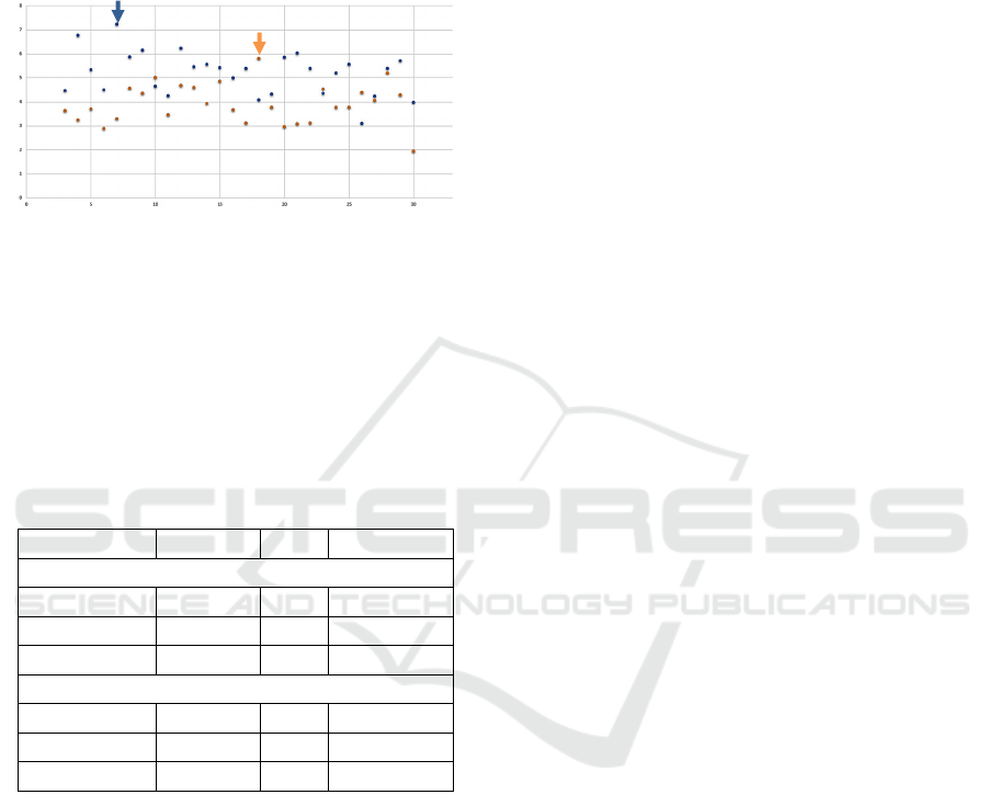
model. The points in the diagram seem to change

their value arbitrarily and further experiments are

needed to evaluate the connections between the

parameter settings and the quality of the resulting

model. The maxima are again indicated by the two

arrows in blue and orange respectively.

Figure 5: SOM: weighted silhouette coefficients for offense

(blue) and defence (orange) data.

4.4.2 Identifying the Clustering Method

After selecting the optimal parameter settings, the

silhouette coefficients of the clustering models have

been compared.

Table 1

gives an overview of the

values in case of the offense and the defence ttms

respectively.

Table 1: Comparison of model quality.

Method s |{c}| ws

Offense

DBSCAN 0.467 18 8.407

Hierarchical 0.497 20 9.943

SOM 0.452 16 7.235

Defence

DBSCAN 0.414 11 4.555

Hierarchical 0.431 13 5.599

SOM 0.415 14 5.812

The overall quality values of the cluster models in

the offense case are significantly greater than the

values of the defence case. Furthermore, the

differences of the quality indicators are significantly

larger in the offense case compared to the defence

case.

The best weighted silhouette coefficient in case of

offense ttms is achieved by Hierarchical Clustering

followed by the DBSCAN method and the Self-

Organizing Maps. In case of the defence data the

SOM has the highest weighted silhouette coefficient

followed by the Hierarchical Clustering and the

DBSCAN approach.

In both cases the Hierarchical Clustering has the

highest non-weighted silhouette coefficient, given the

optimal parameter settings with respect to the

weighted silhouette coefficient, even though the

weighted silhouette coefficient of the SOM approach

is higher in the defence case. None of the approaches

fails completely to find an appropriate clustering

model.

In conclusion, Hierarchical Clustering has been

selected to identify representatives for offense ttms,

while the SOM network is used to cluster defence

ttms.

5 RESULTS AND CONCLUSIONS

5.1 Result Summary

20 clusters spanning 47 records have been identified

using Hierarchical Clustering and a maximum

inconsistency coefficient of 4.52 in the offense case.

From an application perspective it was possible to

identify 11 different team tactical moves that were

represented by the 20 clusters.

14 clusters representing 35 records have been

identified using self-organizing maps and an initial

neighbourhood size of 18 in the defence case. The

clusters were associated with 12 different team

tactical moves by experts.

The differences between clusters that have been

associated with the same team tactical move but

belong to different clusters are still under

investigation. There seem to be only subtle

differences that are not easy to explain for human

experts at this point. Video clips based on the

trajectories of the team tactical moves have been

generated as a basis for the human classification of

representatives.

5.2 Conclusions and Outlook

It has been successfully shown that using the

silhouette coefficient as a concept to determine the

quality of cluster models even in case of clustering

methods that use a different notion of distance is

applicable and allows to compare the clustering

model. Although the silhouette coefficient is difficult

to be used directly, the weighted variant of the

coefficient can be applied easily.

The results presented in this paper must be seen as

a proof of concept rather than a complete study. The

used data are rather small in terms of the number of

extracted ttms. Extracting the ttms and subsequently

processing them using the clustering methods have

shown that the timing accuracy during recording is

crucial. As a side effect the extraction of ttms can be

used to get an indication of the quality of the recorder.

Using the Silhouette Coefﬁcient for Representative Search of Team Tactics in Noisy Data

201

The number of identified team tactical moves

seems to be small but given the small amount of data

it is surprisingly large. From an application

perspective it is far beyond human capabilities to

identify more than 20 different team tactical moves

by the observation of just 5 matches. Furthermore,

handball experts were particularly surprised by the

identified defence tactical moves that the clustering

approach was able to differentiate.

There is still a significant number of parameter

settings that need to be evaluated systematically –

especially in case of the SOMs. Investigating the

SOM settings is particularly time consuming because

the computation of a SOM model takes about a

hundred times longer than the computation done with

other techniques that exploit pre-computed distances.

However, we are very confident that the approach

allows to avoid the need for the manual classification

of thousands of ttms to be able to train a deep learning

network. There will be data of much more matches

available soon when the handball league decides to

share positional data across teams which will allow to

generate a more comprehensive view of played

handball tactics.

ACKNOWLEDGEMENTS

I would like to thank the German Handball League

(HBL) and the teams of TVB Stuttgart, HBW

Balingen-Weilstetten and Frisch Auf! Göppingen for

the support of this work by providing spatiotemporal

data as well as scouting data of matches. Furthermore,

I would like to thank Eckard Nothdurft for

contributing scouting data and for evaluating tactical

video clips to “explain” clusters.

REFERENCES

Aronov, B., Har-Peled, S., Knauer, C., Wang, Y., & Wenk,

C. (2006). Fréchet distance for curves, revisited.

European symposium on algorithms (S. 52-63). Berlin,

Heidelberg: Springer.

Ester, M., Kriegel, H. P., Sander, J., & Xu, X. (1996).

Density-based spatial clustering of applications with

noise. Int. Conf. Knowledge Discovery and Data

Mining, 240, S. 6.

Kinexon. (2017). Real-time Performance Analytics.

Kinexon.

Kumar, V., Chhabra, J. K., & Kumar, D. (2014).

Performance evaluation of distance metrics in the

clustering algorithms. INFOCOMP Journal of

Computer Science, 13(1), S. 38-52.

Martinez, W. L., & Martinez, A. R. (2005). Exploratory

Data Analysis with MATLAB. Boca Raton, Florida:

Chapman & Hall / CRC Press.

MathWorks. (03. 02 2022). MATLAB Help Center. Von

Silhouette Plot:

https://de.mathworks.com/help/stats/silhouette.html

abgerufen

Murtagh, F., & Contreras, P. (2012). Algorithms for

hierarchical clustering: an overview. Wiley

Interdisciplinary Reviews: Data Mining and

Knowledge Discovery, 2(1).

Saitta, S., Raphael, B., & Smith, I. (2008). A

comprehensive validity index for clustering. Intelligent

Data Analysis, 12(6), S. 529-548.

Schwenkreis, F. (2018a). An Approach to use Deep

Learning to Automatically Recognize Team Tactics in

Team Ball Games. Proeedings of the 7th Conference on

Data Science, Technology and Applications. Porto:

Scitepress.

Schwenkreis, F. (2018b). A Three Component Approach

To Support Team Handball Coaches. 23rd Annual

Congress of the European College of Sport Science.

Dublin.

van Hulle, M. (2012). Self-Organizing Maps. In G.

Rozenberg, T. Bäck, & J. N. Kok, Handbook of Natural

Computing (S. 585-622). Berlin, Heidelberg: Springer.

Xu, D., & Tian, Y. (2015). A comprehensive survey of

clustering algorithms. Annals of Data Science, 2(2), S.

165-193.

DATA 2022 - 11th International Conference on Data Science, Technology and Applications

202