Detection, Tracking, and Speed Estimation of Vehicles:

A Homography-based Approach

Kaleb Blankenship and Sotirios Diamantas

Department of Computer Science and Electrical Engineering, Tarleton State University,

Texas A&M University System, Box T-0390, Stephenville, TX 76402, U.S.A.

Keywords:

Object Detection, Multi-object Tracking, Homography Estimation, Speed Estimation.

Abstract:

In this research we present a parsimonious yet effective method to detect, track, and estimate the speed of

multiple vehicles using a single camera. This research aims to determine the efﬁcacy of homography-based

speed estimations derived from details extracted from objects of interest. At ﬁrst, a neural network trained to

detect vehicles outputs bounding boxes. The output of the neural network serves as an input to a multi-object

tracking algorithm which tracks the detected vehicles while, at the same time, their speed is estimated through

a homography-based approach. This algorithm makes no assumptions about the camera, the distance to the

objects, or the direction of motion of vehicles with respect to the camera. This method proves to be accurate

and efﬁcient with minimal assumptions. In particular, only the mean dimensions of a passenger vehicle are

assumed to be known and, using the homography matrix derived from the corners of a vehicle, the speed of

any vehicle in the frame irrespective of its motion direction and regardless of its size is able to be estimated.

In addition, only a single point from each tracked vehicle is needed to infer its speed, avoiding repeatedly

computing the homography matrix for each and every vehicle, thus reducing the time and computational

complexity of the algorithm. We have tested our algorithm on a series of known datasets, the results from

which validate the approach.

1 INTRODUCTION

In this research we demonstrate our ﬁndings from de-

tecting, tracking, and estimating the speed of multiple

vehicles using only a single camera. Estimating the

speed of vehicles, especially on highways, has been

an important topic of research for several decades. In

the last few years, however, there has been a resur-

gence of interest in this ﬁeld due to the imminent ad-

vent of autonomous vehicles. Most of the research in

this ﬁeld relies on Time-of-Flight (ToF) sensors where

a transceiver emits a signal measuring the time it takes

to hit a target vehicle and return to the receiver (Sar-

bolandi et al., 2018), (Li et al., 2013). This method

has been proven accurate, however, there are several

drawbacks. One drawback in particular being that

only one vehicles’ speed can be estimated at a time.

On a highway, there are many vehicles passing at

any moment, and more than one of them may need

attention. Having only one vehicle targeted by a mea-

suring device is not enough as there may be several

vehicles whose speed may need to be estimated. In

addition, the handling of the device needs to be pre-

cise enough to target a vehicle adequately to have

an estimate of its speed as the signal emitted needs

to reach the right vehicle. Line of sight is also an-

other drawback. More speciﬁcally, targeting one ve-

hicle with a ToF device may be occluded or obstructed

by another passing vehicle thus giving erroneous es-

timated of a vehicles’ speed. Finally, ToF sensors es-

timate the speed of a vehicle at a given point in time.

A vehicle’s speed throughout a period of time cannot

be determined.

Other popular methods for estimating vehicles’

speed include piezoelectric sensors embedded into the

ground in two different parts of a road with a known

distance between them, thus the time taken for a vehi-

cle to move from one piezoelectric sensor to the other

is recorded and the speed is, therefore, inferred (Rajab

et al., 2014), (Markevicius et al., 2020). Other similar

approaches for estimating a vehicle’s speed are based

on the use of magneto-resistive sensors (Markevicius

et al., 2017). This method, in spite of its accuracy, suf-

fers also from some major drawbacks. More specif-

ically, if several vehicles cross either the ﬁrst or the

second piezoelectric sensor at the same time, it may

Blankenship, K. and Diamantas, S.

Detection, Tracking, and Speed Estimation of Vehicles: A Homography-based Approach.

DOI: 10.5220/0011093600003209

In Proceedings of the 2nd International Conference on Image Processing and Vision Engineering (IMPROVE 2022), pages 211-218

ISBN: 978-989-758-563-0; ISSN: 2795-4943

211

be difﬁcult to know which estimated speed belongs

to which vehicle. This is the reason this method is

more frequently used in country side roads and less,

if at all, on busy highways. In addition, this method

requires installation of equipment on the ground. Fi-

nally, this method, suffers, too, from calculating a ve-

hicles’ speed at a given point in time, therefore, mak-

ing it impossible to track the speed of a vehicle con-

tinuously in time. A work by (Dailey et al., 2000)

uses assumptions drawn from distributions about the

mean height, width, and length of vehicles.

Computer vision has played an important role in

estimating the speed of vehicles (Hassaballah and

Hosny, 2019). Several methods make use of computer

vision sensors only. In several of these approaches,

assumptions about the environment or the camera

need to be made. For example, in many works, the

computer vision system has to be at a known dis-

tance from the vehicles. This is, in particular, the case

where a camera is placed atop a bridge with a known

height from the ground. Other methods rely on known

marks on the ground or in the image plane. Further-

more, in some instances, the direction of motion plays

an important role in the estimation process. In a work

by (Diamantas and Dasgupta, 2014) the direction of

motion of the vehicle needs to be perpendicular to the

optical axis of the camera.

In this research, our algorithm addresses all of the

above shortcomings yet still provides accurate and

continuous estimates of multiple vehicles using only

a single, non-invasive sensor, that is, a camera. In par-

ticular, our algorithm does not require the installation

of any specialized equipment on the road nor does it

make any assumptions about any known distances to

the target vehicle or the camera. Moreover, it does

not compute the instantaneous speed of a vehicle but

rather it computes and records the speed of a vehi-

cle throughout the whole duration of the video, thus,

providing concrete evidence of a vehicles’ speed and

acceleration which might otherwise be spurious if an

instant estimate is drawn.

Furthermore, the direction of motion of a vehicle

does not affect the speed estimates. Our algorithm

provides precise estimates irrespective of the motion

and direction of the vehicle with respect to the cam-

era. Finally, homography matrix estimation is carried

out once during the initialization process of our al-

gorithm in any one given vehicle, thus, signiﬁcantly

minimizing the computational complexity for contin-

uously computing the homography matrix in every

frame and for every vehicle. Our algorithm has been

tested on several datasets with multiple cars on busy

highways. Additionally, we have also carried out ex-

periments with a known vehicle speed serving as the

ground truth with the view to infer the error in our

approach.

This paper consists of ﬁve sections. In the next

section, background and related works in the ﬁelds

of detection, tracking, and speed estimation are pre-

sented. In Section 3, we present and describe our

methodology as well as the different algorithms en-

compassing our approach for detection, tracking, and

speed estimation. Section 4, presents the results of

our proposed algorithm. Qualitative, as well as quan-

titative results, are provided and compared with the

ground truth. Finally, Section 5 epitomizes our pa-

per with a discussion on the conclusions drawn from

this research as well as the current work that is taking

place and the plans for future work.

2 RELATED WORKS

Tracking many objects simultaneously, especially in

busy difﬁcult environments, and extracting informa-

tion such as height and speed from them over a pe-

riod is, in fact, a multitude of different challenges

wrapped into one. The task of tracking objects alone

requires identifying the object, recognizing the move-

ment and updated locations of objects, and conclud-

ing which object is which at any given point. Individ-

ual aspects of object tracking have seen signiﬁcant re-

search, especially in recent years with research being

spurred by autonomous vehicles. Because so many

challenges construct one singular goal, there can be a

large amount of beneﬁt to the overlap in tying together

multiple systems that solve individual problems.

2.1 Object Detection

You Only Look Once (YOLO) is a darknet-based ob-

ject detector that takes a unique approach to object

detection. Darknet-53 (Redmon, 2021) is the speciﬁc

convolutional neural network used as the backbone

for YOLO v3 and YOLOv4 (Redmon and Farhadi,

2018). Compared to prior object detectors which use

classiﬁers and localizers applied to multiple locations

and at different scales to the image, YOLO applies a

single neural network to the entire image. The im-

age is subdivided into regions or blobs which are an-

alyzed and are given bounding boxes and probabili-

ties for different object classes. This approach allows

predictions to be informed by global context because

the neural network is applied to the entire image at

once. This approach is also many times faster than

classiﬁer-based detectors, allowing for real-time ob-

ject detection.

Because object detectors are typically neural net-

IMPROVE 2022 - 2nd International Conference on Image Processing and Vision Engineering

212

work models, they need to be trained on a dataset.

Microsoft’s Common Objects in Context (COCO) is

one of the leading object recognition datasets. COCO

contains images with complex scenes which have ob-

jects in a natural context (Lin et al., 2015). 91 object

types are deﬁned in the dataset.

2.2 Feature Detection and Tracking

Kanade-Lucas-Tomasi (KLT) point trackers ﬁnd the

best ﬁt linear translation between images by using

spatial intensity information to make the process of

ﬁnding the regression less computationally costly

(Lucas and Kanade, 1981). Minimum eigenvalue fea-

ture detection ﬁnds where large gradient changes in

the image intersect. Corner points become features to

track when the minimum of both computed eigenval-

ues of the gradient is above a set threshold. These cor-

ner points can then be found repeatedly and tracked

from frame to frame. In addition to detection and

tracking, an afﬁne transformation is found between

nonconsecutive frames to identify and potentially re-

ject tracked points that are too dissimilar (Shi and

Tomasi, 1994). KLT point trackers are used broadly

in the ﬁeld of computer vision for camera motion

estimation, video stabilization, and object tracking.

When applying KLT point tracking, points can be lost

because of occlusion, lack of contrast, etc. Because

of this, many tracked features end up short-lived, and

therefore, an additional tracking framework can often

be needed to redetect points of interest.

2.3 Multiple Target Tracking

The uniqueness of different objects of interest is an

important condition to maintain in many tracking sce-

narios. Knowing which object is which can be im-

perative in many instances and applications. Data

association techniques such as global nearest neigh-

bor (GNN) (Konstantinova et al., 2003) and multi-

ple hypothesis trackers (MHT) aim to solve the is-

sue of uniqueness in cluttered environments. Algo-

rithms like these usually employ gating techniques

along with ﬁltering such as Kalman ﬁltering to make

broad decisions before making ﬁner deductions. Var-

ious algorithms are then used to update the identiﬁca-

tions of the tracks (Bardas et al., 2017).

3 METHODOLOGY

This section provides the process and workﬂow be-

hind estimating speed. Speed and depth estimation

are at the summit of a long multifaceted path con-

sisting of ﬁnding objects to track, tracking the ob-

jects which are found, solving for uniqueness, im-

age manipulation, and every hurdle and complica-

tion in-between. Methods that rely on depth appear

in (Diamantas et al., 2010), (Diamantas, 2010). Be-

cause tracking objects and estimating depth is such a

complex challenge, we decided to split it into smaller

more manageable problems, with each step providing

new challenges to solve, not only in it of itself, but

also in order to work with each step of the rest of the

process.

In order to ﬁnd an object’s speed, ﬁrst, where the

object is must be known. For this, object detection

is needed. With current object detection algorithms

arises another challenge, computational power. Ob-

ject detection requires a large amount of computing

resources. If we want to ﬁnd, for example, vehicle

speeds in real-time using easily accessible computing

power, object detection for every new input (frame)

isn’t feasible. It is also quite a waste of resources

when there are much less demanding ways to track

object positions frame-to-frame, such as point track-

ing. An object detector still needs to be run period-

ically to detect new objects and regather points on

already tracked objects, but point tracking or other

tracking algorithms are the frame-to-frame solutions

for tracking changes in object position.

In order to track object speed, ﬁrst, detection of

the object is done, then tracking of changes in ob-

ject position. The next issue arises when we consider

tracking multiple objects. In the case of speed esti-

mation, we must know which object is which. If a car

is being tracked, and a new car appears nearby, there

needs to be a protocol in place to decide which ob-

ject is which from frame to frame and with each new

round of detection. This is another challenge faced on

the way to speed estimation.

3.1 Detection Phase

The ﬁrst step for any tracking or collection of data of

objects of interest is to detect those objects. Object

detection is a rapidly advancing ﬁeld in computer sci-

ence, and there are many different detectors out there.

One thing most modern detectors have in common is

that they are neural network models, but beyond that,

the structure, design, and techniques used can vary

greatly.

For this project, we decided to implement

YOLOv4 in this detection algorithm. YOLO was the

detector of choice because of its balance of detec-

tion accuracy and detection speed. One of the pri-

mary goals in speed estimation is for it to be real-time.

Detection, Tracking, and Speed Estimation of Vehicles: A Homography-based Approach

213

YOLOv4 achieves 43.5% AP (65.7% AP50) on the

MS COCO dataset with a speed of roughly 65 frames

per second using a Tesla V100 graphics card. Com-

pared to EfﬁcientDet, another state-of-the-art detec-

tor, YOLO boasts twice the detection speed at com-

parable accuracy (Bochkovskiy et al., 2020).

Using code to import the YOLO models to MAT-

LAB (YOLOv4, 2021), YOLOv4 is periodically run

to detect new objects and recollect features on already

tracked objects. In much of our testing, 500 mil-

lisecond intervals proved to be an appropriate interval

rate for real-time operation, quick detection of newly

presented objects, and consistent point recollection.

YOLO produces axis-aligned bounding boxes for all

detected objects as well as categories and conﬁdence

values for each detection. Objects with a conﬁ-

dence value over a certain threshold are kept. Non-

maximum suppression (NMS) keeps objects from be-

ing double-counted.

3.2 Tracking and Data Collection Phase

In order to progress from object detection to object

tracking, a few issues need to be addressed. Firstly, in

multi-object tracking, the uniqueness of each object

needs to be maintained. In other words, when tracking

multiple objects, knowing which object is which is

important. Second, in-between detections being run,

the movement of objects needs to be tracked and their

bound boxes adjusted accordingly. Lastly, because

the view of objects can in many cases be temporarily

obstructed and because some objects may be difﬁcult

to detect, predicting the future position of tracks can

be utilized to produce more consistent tracking and

allows the tracking to be more robust in many more

challenging situations.

There are a number of approaches for deducing

which object is which. We chose a ranked assign-

ment method (Murty, 1968) which uses a cost matrix

to determine assignments with the least cost. The op-

timized ranked assignment method we implemented

greatly optimizes the method by partitioning in an op-

timized order, inheriting partial solutions, and sorting

sub-problems (Miller et al., 1997).

Utilizing a KLT algorithm (Tomasi and Kanade,

1991) with the bounding boxes provided by object

detection as the region of interest, we were able to

get consistent feature extraction and tracking (Shi and

Tomasi, 1994). Since the objects of interest were of-

ten moving objects, we used bidirectional error along-

side point tracking to determine and eliminate points

detached from the objects being tracked (Kalal et al.,

2010). With these measures in place, points that

proved to be quality points on the object to track were

then used to interpolate the object’s change in position

from frame to frame. The interpolation arises from

the geometric transform estimation derived from the

points’ change in position between frames (Torr and

Zisserman, 2000).

For predictions and data collection, a Kalman ﬁl-

ter for each bounding box continually updates with

the current position of the midpoint of the bottom

edge of each bounding box. With the path of this point

being fed to the Kalman ﬁlter, the Kalman ﬁlter can

then predict, in a linear fashion, the future positions

of this point (Welch and Bishop, 2006). This point

serves two purposes. Its ﬁrst purpose is as a reference

from which the bounding box can be reconstructed

when the object is lost. If an object is a particularly

difﬁcult detection or if an object is temporarily oc-

cluded, all tracked points can be lost. In a short time,

if a new detection is found which matches the pre-

dicted position of a lost track, we can say with some

conﬁdence this is the same object. The Kalman ﬁl-

tered point’s second purpose will be discussed in the

next subsection. Variations of an extended Kalman

ﬁlter could be implemented for more advanced pre-

dictions (Simon, 2006), but because the conﬁdence

of an object reappearing drastically reduces quickly

in most scenarios we presented, the computationally

light basic Kalman ﬁlter was used.

3.3 Homography-based Speed

Estimation

Speed estimation lies at the summit of this algorithm.

Although the large push for autonomous vehicles has

caused greatly accelerated advancements in computer

vision, speed estimation and 3D scene recreation have

continued to be very challenging topics. More and

more complex techniques for data collection such as

lidar and multi-camera systems have come to the fore-

front of depth perception research, but many of these

techniques are expensive, inaccessible, or too inva-

sive a solution in certain environments with certain

constraints. There is a need to create a robust speed

estimation algorithm that needs very minimal infor-

mation to work reliably.

The biggest hurdle in speed estimation with a sin-

gle camera is projecting a 3D scene from a 2D repre-

sentation, i.e. an image, in a meaningful way to then

gather speed. Many ways of doing this have the ba-

sic requirement of knowing the camera’s extrinsic pa-

rameters such as pose and height. In many scenarios,

extrinsics like this are unknown and difﬁcult to ﬁnd.

Making the simple assumptions that 1) the ground in

the scene is ﬂat and 2) the objects you are tracking

are moving along the ground, planar homography can

IMPROVE 2022 - 2nd International Conference on Image Processing and Vision Engineering

214

be used to shift the perspective of the image in a way

which speed can then be extracted. Homography is a

bijective isomorphism of a projective space. Homog-

raphy is traditionally used for image rectiﬁcation and

computation of camera motion between images.

The question then arises, how do we ﬁnd the ho-

mography transform of an image in order to ﬁnd the

speed of vehicles and the like? First, a set of points

parallel to the ground plane is needed with known

mappings to real-world distances. Keeping in mind

the primary goal in this paper is to monitor vehicle

speed, points from passing vehicles can be collected

and used as the foundation for a homography matrix

derivation. In this work, four corners of a passing ve-

hicle, where the headlights and tail lights are located,

were manually picked during the initialization of the

algorithm. Lastly, using these points along with the

average dimensions of a vehicle, we were able to con-

sistently produce an image transformation productive

for speed estimation utilizing planar homography in

MATLAB (Corke, 2017). Assuming the ground is rel-

atively ﬂat, the transformed image acts essentially as

a Bird’s Eye View where pixel-wise distances on the

same plane as the ground are known. For each ob-

ject, the midpoint of the bottom bounding box edge,

where the vehicle meets the ground plane, discussed

in section 3.2 can be processed though the homogra-

phy transformation matrix. The changes in the po-

sition of the now transformed midpoints can then be

mapped to real world distances. The homography ma-

trix H transforms the set of points (x

, y

) to set of

points (x

, y

H =









(1)









= H

























(2)

+ h

) = h

+ h

(3)

+ h

) = h

+ h

(4)

8 degrees of freedom can safely be enforced by setting

to 1:

+ h

+ 1

(5)

+ h

+ 1

(6)

From this derivation, further corresponding sets of

points can be included to ﬁt a homography matrix to

all points. The corners of a reference vehicle and the

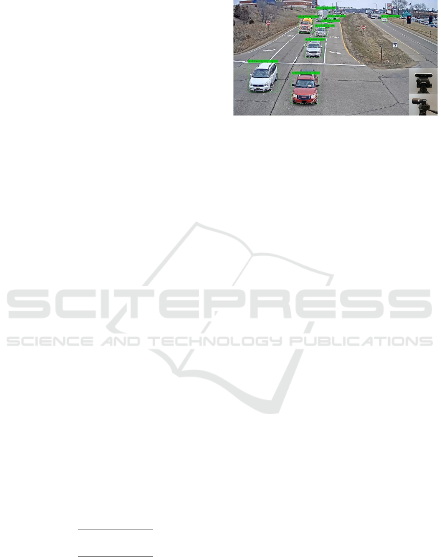
Figure 1: A sample image from a dataset showing detected,

tracked, and speed estimates of various vehicles’ sizes. In

the lower right corner, two of the camera sensors used in

experiments with self-owned vehicle are shown.

average dimensions of a vehicle where used to com-

pute the transformation matrix of the image. Thus,

having computed the homography matrix, the follow-

ing equation (7) is used to estimate the speed between

consecutive frames:

v(t) =

∆s

∆t

(7)

where ∆t is given by the extracted frame rate

of the camera. With an appropriate camera angle

paired with YOLO’s ability to distinguish between

cars, trucks, and buses, semantic segmentation (J

egou

et al., 2017) and optical ﬂow techniques could be used

to automate point acquisition during the initialization

process, and, further, repeatedly ﬁnd transformations

from passing vehicles, allowing for a further rectiﬁed

transformation matrix over time, or even allow for a

moving camera (Diamantas and Alexis, 2020), (Dia-

mantas and Alexis, 2017).

In Fig. 1 various detected and tracked vehicles

(passenger cars, trucks, large trucks) along with their

estimated speed is shown. In the lower right corner

the sensors (FLIR Blackﬂy and Intel Realsense D455)

used for the experiments are also depicted.

4 EXPERIMENTS AND RESULTS

The following ﬁgures present experimental work with

videos taken from datasets as well as videos created

with a self-owned vehicle that served as a ground truth

to compute the error in estimated speeds. Figure 2

shows the output of the algorithm using datasets with

different videos. Each column contains vehicles go-

ing in different directions. This algorithm is robust to

scale as well as to motion direction of vehicles. Fig-

ure 3 shows images with a self-owned vehicle and a

known speed. The error has been estimated to be as

low as 0.3 km/h and as high as 7.5 km/h in some few

Detection, Tracking, and Speed Estimation of Vehicles: A Homography-based Approach

215

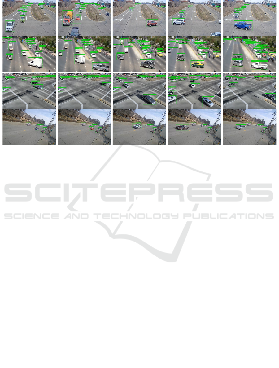
Figure 2: Output of proposed algorithm. Speed estimations of a number of vehicles with various sizes moving into different

directions validate the effectiveness of our proposed algorithm. Videos from different data sets have been used in this set of

experiments.

instances. In most experiments the error is between

3-5 km/h. Figure 4 images have been taken using

a smartphone camera. In this experiment, the error

lies within the afore-mentioned range. The resolution

of frames varies with most videos having a resolu-

tion of 1920 × 1080 and in one case, a resolution of

2560 × 1920 (Fig. 2, last row). The frame rate varies

between 10 fps and 50 fps. In all different settings

our algorithm performed remarkably well. The source

code of our approach is available at Github

. Several

videos with the output of our algorithm can be found

on our YouTube channel

5 CONCLUSIONS AND FUTURE

WORK

In this research, we have presented an algorithm for

detecting, tracking, and estimating the speeds of mul-

tiple vehicles. In particular, this method comprises of

several sub-algorithms, at ﬁrst a neural network algo-

rithm, based on YOLOv4, detects multiple vehicles

on the highway which in turn serves as input to a

multiple-object tracker based on the KLT algorithm.

Using the homography matrix, which is computed

only once based on the mean dimensions of passenger

https://github.com/TSUrobotics/SpeedEstimation

https://www.youtube.com/channel/

UCeyQfeblSg2eyX2gGSUpIOw

vehicles and the four corners of any passenger vehicle

at the beginning of our video, we are able to estimate

and track the speed of all vehicles for the entire dura-

tion of the video. This algorithm requires only a sin-

gle feature from any vehicle to be tracked in order to

infer its speed. The algorithm is, thus, computation-

ally cheap yet it provides accurate estimates of vehi-

cles’ speeds irrespective of the direction of motion of

vehicles or their size. The results validate our algo-

rithm which is tested on a series of known datasets as

well as compared with ground truth data.

The vehicle corner-based homography derivation

could be expanded in a number of ways. One sig-

niﬁcant development would be automating the cor-

ner collection and repeatedly applying it. This would

eliminate any initialization procedure, and allow for

a homography derivation which improves with time.

With some modulation, the methods of this work

could be expanded and applied along with automated

corner collection of vehicles to not only provide much

more accurate speed estimation, but also allow for

speed estimation from a moving camera with very

minimal assumptions.

Currently, we are developing methods to detect

vehicles using semantic segmentation which will pro-

vide an even more accurate estimate of the homog-

raphy matrix. As a future work, we plan on testing

future iterations of this algorithm on a moving vehi-

cle with the aim to estimate the time to collision as

well as to run our algorithm on a parallel processor

IMPROVE 2022 - 2nd International Conference on Image Processing and Vision Engineering

216

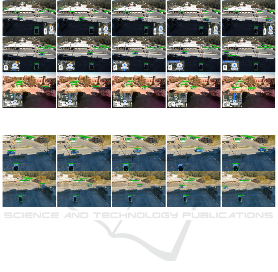
Figure 3: Output of proposed algorithm. In these set of images controlled experiments have been carried out with a self-owned

vehicle with the view to estimate the error.

Figure 4: Output of proposed algorithm. Images are taken by a smartphone camera and a self-owned vehicle is driven with

the view to estimate the error.

platform. Moreover, we plan on combining the cur-

rent approach with optical ﬂow techniques with the

view to provide more robust results especially in sce-

narios where a vehicle is stopped and a small amount

of speed is estimated with the proposed algorithm.

Finally, we plan on implementing this approach on

an Unmanned Aerial Vehicle (UAV) and use thermal

camera imaging to infer speeds at night.

REFERENCES

Bardas, G., Astaras, S., Diamantas, S., and Pnevmatikakis,

A. (2017). 3D tracking and classiﬁcation system using

a monocular camera. Wireless Personal Communica-

tions, 92(1):63–85.

Bochkovskiy, A., Wang, C.-Y., and Liao, H.-Y. M. (2020).

Yolov4: Optimal speed and accuracy of object detec-

tion. arXiv:2004.10934.

Corke, P. I. (2017). Robotics, Vision & Control: Fundamen-

tal Algorithms in MATLAB. Springer, second edition.

ISBN 978-3-319-54413-7.

Dailey, D. J., Cathey, F. W., and Pumrin, S. (2000). An

algorithm to estimate mean trafﬁc speed using uncal-

ibrated cameras. IEEE Transactions on Intelligent

Transportation Systems, 1(2):98–107.

Diamantas, S. and Alexis, K. (2017). Modeling pixel in-

tensities with log-normal distributions for background

subtraction. In 2017 IEEE International Conference

on Imaging Systems and Techniques (IST), pages 1–6.

Diamantas, S. and Alexis, K. (2020). Optical ﬂow based

background subtraction with a moving camera: Ap-

plication to autonomous driving. In et al, G. B., edi-

tor, Advances in Visual Computing. ISVC 2020. Lec-

ture Notes in Computer Science, volume 12510, pages

398–409. Springer.

Diamantas, S. C. (2010). Biological and Metric Maps

Applied to Robot Homing. PhD thesis, School

of Electronics and Computer Science, University of

Southampton.

Diamantas, S. C. and Dasgupta, P. (2014). Active vi-

sion speed estimation from optical ﬂow. In et al,

A. N., editor, Towards Autonomous Robotic Systems,

TAROS 2013, Revised Selected Papers, Lecture Notes

in Artiﬁcial Intelligence, volume 8069, pages 173–

184. Springer Berlin Heidelberg.

Detection, Tracking, and Speed Estimation of Vehicles: A Homography-based Approach

217

Diamantas, S. C., Oikonomidis, A., and Crowder, R. M.

(2010). Depth computation using optical ﬂow and

least squares. In 2010 IEEE/SICE International Sym-

posium on System Integration, pages 7–12, Sendai,

Japan.

Hassaballah, M. and Hosny, K. (2019). Recent Ad-

vances in Computer Vision: Theories and Applica-

tions. Springer, Cham.

egou, S., Drozdzal, M., Vazquez, D., Romero, A., and

Bengio, Y. (2017). The one hundred layers tiramisu:

Fully convolutional densenets for semantic segmenta-

tion. arXiv:1611.09326.

Kalal, Z., Mikolajczyk, K., and Matas, J. (2010). Forward-

backward error: Automatic detection of tracking fail-

ures. In In Proceedings of the 2010 20th International

Conference on Pattern Recognition, ICPR ’10, pages

2756–2759. IEEE Computer Society.

Konstantinova, P., Udvarev, A., and Semerdjiev, T. (2003).

A study of a target tracking algorithm using global

nearest neighbor approach. International Conference

on Computer Systems and Technologies - CompSys-

Tech’2003.

Li, C., Chen, Q., Gu, G., and Qian, W. (2013). Laser time-

of-ﬂight measurement based on time-delay estimation

and ﬁtting correction. Optical Engineering, 52(7).

Lin, T.-Y., Maire, M., Belongie, S., Bourdev, L., Girshick,

R., Hays, J., Perona, P., Ramanan, D., Zitnick, C. L.,

and Doll

ar, P. (2015). Microsoft coco: Common ob-

jects in context. arXiv:1405.0312.

Lucas, B. D. and Kanade, T. (1981). An iterative image

registration technique with an application to stereo vi-

sion. In Proceedings of the 7th International Joint

Conference on Artiﬁcial Intelligence (IJCAI), August

24-28, pages 674–679.

Markevicius, V., Navikas, D., Idzkowski, A., Valinevicius,

A., Zilys, M., and Andriukaitis, D. (2017). Vehi-

cle speed and length estimation using data from two

anisotropic magneto-resistive (amr) sensors. Sensors,

17(8):1–13.

Markevicius, V., Navikas, D., Miklusis, D., Andriukaitis,

D., Valinevicius, A., Zilys, M., and Cepenas, M.

(2020). Analysis of methods for long vehicles speed

estimation using anisotropic magneto-resistive (amr)

sensors and reference piezoelectric sensor. Sensors,

20(12):1–15.

Miller, M. L., Stone, H. S., , Cox, I. J., and Cox, I. J. (1997).

Optimizing murty’s ranked assignment method. IEEE

Transactions on Aerospace and Electronic Systems,

33:851–862.

Murty, K. G. (1968). An algorithm for ranking all the as-

signments in order of increasing cost. Operations Re-

search, 16(3):682–687.

Rajab, S. A., Mayeli, A., and Refai, H. H. (2014). Vehi-

cle classiﬁcation and accurate speed calculation using

multi-element piezoelectric sensor. In 2014 IEEE In-

telligent Vehicles Symposium (IV), pages 894–899.

Redmon, J. (2021). Darknet: Open source neural networks

in c. http://pjreddie.com/darknet/.

Redmon, J. and Farhadi, A. (2018). Yolov3: An incremental

improvement. arXiv:1804.02767.

Sarbolandi, H., Plack, M., and Kolb, A. (2018). Pulse based

time-of-ﬂight range sensing. Sensors, 18(6):1–22.

Shi, J. and Tomasi (1994). Good features to track. In 1994

Proceedings of IEEE Conference on Computer Vision

and Pattern Recognition, pages 593–600.

Simon, D. (2006). Optimal state estimation: Kalman, h

inﬁnity, and nonlinear approaches. In Optimal State

Estimation: Kalman, H Inﬁnity, and Nonlinear Ap-

proaches. Wiley-Interscience.

Tomasi, C. and Kanade, T. (1991). Shape and motion from

image streams: a factorization method – part 3 detec-

tion and tracking of point features. Technical Report

CMU-CS-91-132, Carnegie Mellon University, Pitts-

burgh, PA.

Torr, P. and Zisserman, A. (2000). Mlesac: A new ro-

bust estimator with application to estimating image

geometry. Computer Vision and Image Understand-

ing, 78(1):138–156.

Welch, G. and Bishop, G. (2006). An introduction to the

kalman ﬁlter. Technical Report TR 95-041, Depart-

ment of Computer Science, University of North Car-

olina at Chapel Hill, Chapel Hill, NC, USA.

YOLOv4 (2021). https://github.com/cuixing158/yolov3-

yolov4-matlab.

IMPROVE 2022 - 2nd International Conference on Image Processing and Vision Engineering

218