Analysis of Incremental Learning and Windowing to Handle Combined

Dataset Shifts on Binary Classiﬁcation for Product Failure Prediction

Marco Spieß

, Peter Reimann

1,2

, Christian Weber

and Bernhard Mitschang

Graduate School of Excellence advanced Manufacturing Engineering (GSaME), University of Stuttgart, Germany

Institute for Parallel and Distributed Systems (IPVS), University of Stuttgart, Germany

bernhard.mitschang}@ipvs.uni-stuttgart.de

Keywords:

Binary Classiﬁcation, Combined Dataset Shift, Incremental Learning, Product Failure Prediction, Windowing.

Abstract:

Dataset Shifts (DSS) are known to cause poor predictive performance in supervised machine learning tasks.

We present a challenging binary classiﬁcation task for a real-world use case of product failure prediction. The

target is to predict whether a product, e. g., a truck may fail during the warranty period. However, building

a satisfactory classiﬁer is difﬁcult, because the characteristics of underlying training data entail two kinds

of DSS. First, the distribution of product conﬁgurations may change over time, leading to a covariate shift.

Second, products gradually fail at different points in time, so that the labels in training data may change,

which may a concept shift. Further, both DSS show a trade-off relationship, i. e., addressing one of them may

imply negative impacts on the other one. We discuss the results of an experimental study to investigate how

different approaches to addressing DSS perform when they are faced with both a covariate and a concept shift.

Thereby, we prove that existing approaches, e. g., incremental learning and windowing, especially suffer from

the trade-off between both DSS. Nevertheless, we come up with a solution for a data-driven classiﬁer, that

yields better results than a baseline solution that does not address DSS.

1 INTRODUCTION

Dataset Shifts (DSS) (Qui

nonero-Candela et al.,

2008) relate to the phenomenon that properties

and statistical distributions of data change over

time (Moreno-Torres et al., 2012). They are com-

mon in many real-world application scenarios of non-

stationary environments and their study is an active

area of research (Ditzler et al., 2015; Bang et al.,

2019; Dharani Y. et al., 2019; Losing et al., 2018;

Elwell and Polikar, 2011). Literature discusses vari-

ous types of DSS (Moreno-Torres et al., 2012). Es-

pecially two types of DSS occur more frequently in

practice than others and are therefore of particular rel-

evance: a covariate shift (Dharani Y. et al., 2019) and

a concept shift (Elwell and Polikar, 2011). A covari-

ate shift is a shift in the distribution of feature values

between a training dataset T and a test dataset T

, so

that single class patterns occur with different frequen-

cies. A concept shift constitutes a change in the deci-

sion boundaries of individual class patterns. Usually,

DSS cause poor prediction performance in supervised

machine learning tasks (Kull and Flach, 2014).

Related work proposes approaches such as incre-

mental learning (Losing et al., 2018) and window-

ing (Bifet and Gavald

a, 2007) to address either co-

variate or concept shifts. Moreno-Torres et al. high-

light that no adequate solution exists that addresses

combinations of both kinds of DSS, since such com-

binations seem to be rare in practice (Moreno-Torres

et al., 2012). However, data of many real-world use

cases, e. g., from product design (Nalbach et al., 2018)

or medical diagnoses (Khan and Usman, 2015; Mait

ın

et al., 2020), often suffer from both DSS. Here, such

combined DSS make it difﬁcult to build classiﬁers for

improving product design and automating medical di-

agnoses. So far, no studies investigate how different

approaches for dealing with DSS perform when con-

fronted with both covariate shifts and concept shifts.

In this paper, we analyze approaches to deal with

combined dataset shifts. To this end, we have devel-

oped a real-world use case together with a large global

truck manufacturer. The manufacturer ﬁnds that an

increased number of trucks suddenly fail during the

warranty period. A root cause analysis shows that the

targeted assembly of more robust product components

prevents these failures. Accordingly, the truck manu-

394

Spieß, M., Reimann, P., Weber, C. and Mitschang, B.

Analysis of Incremental Learning and Windowing to Handle Combined Dataset Shifts on Binary Classiﬁcation for Product Failure Prediction.

DOI: 10.5220/0011093300003179

In Proceedings of the 24th International Conference on Enterprise Information Systems (ICEIS 2022) - Volume 1, pages 394-405

ISBN: 978-989-758-569-2; ISSN: 2184-4992

facturer plans to selectively assemble robust parts in

those trucks that are likely to fail. This can be framed

as a supervised machine learning task for product fail-

ure prediction to avoid future failures.

For this task, we collect a training dataset T , rep-

resenting trucks that are already in customer use. The

feature set of T corresponds to the truck conﬁgu-

rations, while a label indicates whether a truck has

failed during the warranty period. The goal is to

learn a binary classiﬁer in order to apply it on a test

dataset T

. This test set T

represents new trucks

and their conﬁgurations that will soon be produced.

The classiﬁer predicts which of these new trucks are

also likely to fail with the less robust components.

The manufacturer then assembles more robust com-

ponents into these trucks as a preventive measure.

Learning the binary classiﬁer is complex because the

use case data characteristics exhibit two types of DSS.

Covariate Shift (CS1): The training data T consists

of 3,000 features that represent the various compo-

nents assembled in each truck. However, the truck

manufacturer produces a large number of truck vari-

ants whose components and conﬁgurations change

over time. This induces a covariate shift (CS1).

Concept Shift (CS2): Trucks may fail at different

points in time during their use phase. Hence, the la-

bels of trucks that eventually fail gradually shift from

”nonfailed” to ”failed” over time, i. e., one truck af-

ter the other. This leads to a concept shift (CS2).

In this paper, we investigate how to build a clas-

siﬁer with satisfactory prediction performance mea-

sured as True-Positive-Rate (TPR) under the inﬂuence

of these two types of dataset shifts in combination.

We thereby make the following main contributions:

• We shed light into real-world data characteristics

and causes of combined DSS in a use case of

product failure prediction. We propose four meta-

features that clearly analyze the extents of covari-

ate (CS1) and concept shifts (CS2) in these data.

• We show that existing approaches to Data Stream

Mining that handle DSS, e. g., incremental learn-

ing and windowing, suffer from a trade-off re-

lationship between covariate (CS1) and concept

shifts (CS2). With our meta-features, it is pos-

sible for the ﬁrst time to measurably analyze the

trade-off behavior of this combined dataset shift.

• We come up with a classiﬁer that yields better re-

sults than a baseline that does not explicitly ad-

dress DSS. This classiﬁer ﬁnally increases the

True-Positive-Rate and leads to a signiﬁcant re-

duction of warranty claim costs by ∼ 13%-points.

01/01/2015

01/01/2017

12/31/2017

2015

2016

2017

…

Quarterly samples from the ongoing production of trucks

Training samples

Test samples

Training

Dataset T

Test

Dataset T‘

Predictive Modeling

Evaluation of Predictions

Classification

Algorithm

Figure 1: Overview on datasets for training and testing pos-

sible classiﬁers that can predict product failures of trucks.

• As basis for our evaluation, we have generated

synthetic datasets. We provide these datasets in

a GitHub repository

to increase reproducibility.

Our paper is structured as follows: in Section 2,

we describe the use case of predicting product failures

and the two kinds of DSS. We discuss related work

in Section 3. Section 4 then illustrates the design of

our experimental study. In Section 5, we discuss the

evaluation results and come up with the classiﬁer that

outperforms the baseline. We conclude in Section 6.

2 DATASET SHIFTS IN PRODUCT

FAILURE PREDICTION TASKS

In this section, we present our use case for product

failure prediction (2.1), describe the underlying data

characteristics (2.2), and how this leads to a covariate

and a concept shift (2.3). Last, we discuss in which

other domains both kinds of DSS occur together (2.4).

2.1 Real-world Use Case from Industry:

Prediction of Product Failures

A truck manufacturer provided us with data from a

real-world use case. The truck manufacturer noticed

that powertrain failures happened more frequently

since the production year 2015. Usually, compo-

nents from the powertrain, e. g., injection pumps, tur-

bocharger, gears, etc. fail due to higher loads. To

therefore avoid possible real-world hints and to in-

crease readability, this paper considers an unspeciﬁed

component from the powertrain. In order to tackle this

quality problem, the truck manufacturer substituted

this component with another more robust one. We

call the initial, less robust part A and its more robust

https://github.com/MarcoS89-dev/Combined-DataSet

Shifts-in-ProductFailurePrediction

Analysis of Incremental Learning and Windowing to Handle Combined Dataset Shifts on Binary Classiﬁcation for Product Failure

Prediction

395

variant B. Starting from 01/01/2017, B is ready for

assembly in trucks and prevents particular powertrain

damages in the later use phase of trucks. However,

due to supply bottlenecks, the availability of part B is

restricted and can only be assembled in a maximum

of 50% of all trucks. Figure 1 shows the correspond-

ing production time line for the use case and which

data we used as training (T ) and test dataset (T

Quality engineers found that individual truck con-

ﬁgurations somehow inﬂuence the proneness to pow-

ertrain damages. The idea is to determine which con-

ﬁgurations are more prone to this damage. So, these

trucks are then assembled with the more robust part

B. Otherwise, part A and B are assembled randomly.

The manufacturer asked data scientists to collect

historical training data and to learn a classiﬁer that

can predict truck failures. On 01/01/2017, the data

scientists built a classiﬁer using the collected training

dataset T of trucks produced in 2015 and 2016 (see

Figure 1). They then applied this classiﬁer to the new

trucks produced in 2017 to decide whether to assem-

ble part A or B in these new trucks. Some years later,

in 2022, the labels in the test data T

have changed

and now show stable class patterns and ﬁxed deci-

sion boundaries. So, the data scientists ﬁnally eval-

uated their classiﬁer in this year again. The evalua-

tion shows a True-Positive-Rate (TPR) of only 55.9%.

This is an increment of 5.90%-points compared to the

random assembly of A and B. However, this 55.9%

is a poor predictive performance and not satisfactory

at all. The data scientists assume that it is due to DSS.

Research goal. This use case provides the starting

point for our study. We investigate different well-

known approaches from Data Stream Mining that ad-

dress DSS. The ultimate goal is to determine if it is

possible to build a classiﬁer that outperforms the base-

line with 55.9% TPR. Please note that the ﬁnal TPR

is only known when enough time has passed. This

means in our case, when each truck from the test data

has completed its warranty period. Thus, we are look-

ing from today’s perspective, i. e., from 2022, into the

past. With this retrograde analysis, we examine if it is

possible to learn a better classiﬁer with different com-

binations of sampling techniques and algorithms.

2.2 Data Characteristics

Table 1 shows the attributes of T and T

: truck iden-

tiﬁcation number, a class label and the feature space

X . The label of a sample is either ”failed” as positive

class c

or ”nonfailed” as negative class c

−

. More-

over, T and T

include only trucks with part A, be-

cause only these may fail due to the particular failure.

Table 1: Exemplary structure of datasets T and T

Truck-

Class

label

Engine

Other

/ c

−

) ABC XYZ part

1 failed 1 0 0

2 nonfailed 0 1 0

3 nonfailed 1 0 1

... ... ... ... ...

Note that the manufacturer only gets data of failed

trucks if the customer brings them to a workshop that

is under contract with the manufacturer. Within the

36-month warranty period, the customer is restricted

to bring his or her trucks to those contracted work-

shops to claim warranty obligations. However, after

the warranty period has expired, the customer is free

to choose another workshop. In this case, we cannot

capture any more labels for trucks out of warranty.

The feature space X is one-hot encoded and con-

tains around 3,000 disjunctive features. So, X con-

sists of η binary variables x

to x

. Each variable rep-

resents one particular truck equipment, e. g., a certain

type of an engine. The binary values 1 and 0 describe

whether a respective equipment is present in a truck

or not. Example: truck 1 and truck 3 in Table 1 are

equipped with an ABC engine, whereas truck 2 has an

XYZ engine. Each truck consists on average of about

186 binary 1’s in X and about 2,814 binary 0’s. The

number of 1’s per truck ranges from 131 to 262.

Meta-features. Table 2 shows the four relevant meta-

features: c

ratio, MIS, V S and V S

With our proposed meta-features, we analyze the

datasets T and T

at two time points: on 01/01/2017

and on 01/01/2022. We use these two different data

states in Section 2.3 to illustrate the DSS of our

datasets. The training set T contains 80,948 trucks

that have been produced in 2015 (T

2015

) or 2016

2016

). On 01/01/2017, only 97 of them have already

failed and thus get the positive class c

as label. As

a result, the c

ratio, which represents the share of

failed trucks to all trucks, is 0.12%. The Months-In-

Service (MIS) (see Table 2) is the operating time of

a truck and correlates with the c

ratio because the

older a truck, the higher its risk of failure.

The trucks in T and T

may differ considerably.

We have identiﬁed 489 key features that describe a

truck in its basic characteristics. These 489 key fea-

tures split into 11 non-overlapping feature domains,

e. g., engine (29 key features), gearbox (30 key fea-

tures), and axle (41 key features). In each feature

domain, we compare the distributions of key features

between T and T

to develop the meta-feature Truck

Similarity V S as a similarity indicator. Truck Similar-

ity V S is the mean of the frequency differences across

ICEIS 2022 - 24th International Conference on Enterprise Information Systems

396

Table 2: View on T and T

on 01/01/2017 and 01/01/2022 with number of trucks (N), failures (c

) and the meta-features.

Set N c

ratio MIS V S V S

Data Status on 01/01/2017

T 80,948 97 0.12% 10.28 79.67% 49.95%

2015

38,659 82 0.21% 16.63 76.73% 49.06%

2016

42,289 15 0.04% 5.29 82.28% 57.40%

Data Status on 01/01/2022

T 80,948 7,245 8.95% 71.89 79.67% 65.14%

42,260 4,585 10,85% 52.11 - -

Table 3: Exemplary comparison of the proportions of key

features within the engine domain between T and T

Key Features

Proportions in...

Difference

T T

H290, 10.8l 17% 12% 5%

H310, 12.9l - 25% 25%

H460, 15.7l 35% 20% 15%

M130, 5.2l 7% 7% 0%

M175, 7.8l 4% - 4%

... ... ... ...

the respective key features. For instance, a particular

engine may be assembled more often or less in T than

in T

, leading to a shift of the frequencies of this par-

ticular feature value. This shift in feature frequencies

and the resulting differences are illustrated in Table 3.

Finally the value of meta-feature V S (see Table 2)

is the result from 100% − di f f erences of all eleven

unweighted feature domains. In order to measure the

truck similarity only between failed trucks from the

training (T ) and the test (T

) datasets, we developed

V S

as the Truck Similarity of Class c

. The calcu-

lation of V S

is the same as for V S , except that we

only use the distributions of failed trucks (c

2.3 Dataset Shifts

The characteristics of our use case and of its data es-

tablish a non-stationary environment that entails two

kinds of dataset shifts for product failure predictions.

For the mathematical description of the DSS we de-

note x as the input variables, i. e. features, and y as the

target class variable (Moreno-Torres et al., 2012).

Covariate Shift (CS1): P

train

(y|x) = P

test

(y|x) and

train

(x) 6= P

test

(x). The functional relationship f (x)

between training and test data remains the same over

time. However, the distributions within the feature

sets x of training and test data are different. Con-

sequently, important class patterns in the test data

may be underrepresented in the training data and vice

versa. This may usually result in a degradation of the

classiﬁcation performance, since relevant class pat-

terns in the test dataset cannot be entirely learned by

a classiﬁcation algorithm from the training dataset.

CS1 occurs in our use case because the conﬁgu-

rations of trucks especially vary for different areas of

application, e. g., construction site or transport trucks.

Over individual quarters, different customers order

different ﬂeets of trucks, which can vary signiﬁcantly

in terms of their areas of application and thus in their

conﬁgurations. Therefore, the trucks in the training

dataset T may differ from those in the test dataset T

This can be seen by the meta-feature V S reported in

Table 2. The value of

80% indicates that the dis-

tribution of feature values in T and T

differ by at

least 20%. Even worse, the similarity of failed trucks

(V S

) is only about 50%. This difference in the dis-

tribution of features constitutes a covariate shift.

Concept Shift (CS2): P

train

(y|x) 6= P

test

(y|x) and

train

(x) = P

test

(x). The distributions of features re-

main the same between training and test data, but a

shift in the mapping function f (x) occurs. This may

usually result in a degradation of the classiﬁcation

performance, since the descriptions of the class pat-

terns change over time, although the feature space X

remains the same. This means that the patterns in the

training data are described either by different features

or value ranges than the actual patterns in the test data.

CS2 occurs in our use case because each sample

of T is initially an element of c

−

(”nonfailed”) and

has a chance to eventually become an element of c

(”failed”). On 01/01/2017, the average MIS of the

80,948 trucks in training data T is about 10 months,

and 97 of them failed so far. Until 01/01/2022, when

the average MIS is about 72 months, the number of

failed trucks increases to 7,245. So, the class label of

7,148 trucks has shifted from c

−

to c

, so that the c

ratio increases from 0.12% to 8.95%. This causes a

concept shift, as the decision boundaries of class pat-

terns may change with each label shift.

Combination of both Shifts CS1 and CS2:

train

(y|x) 6= P

test

(y|x) and P

train

(x) 6= P

test

(x).

Moreno et al. currently consider this combined DSS

Analysis of Incremental Learning and Windowing to Handle Combined Dataset Shifts on Binary Classiﬁcation for Product Failure

Prediction

397

as impossible to solve. Further, they consider that

this DSS is not discussed in literature because it

rarely occurs in practice (Moreno-Torres et al., 2012).

However, in real-world applications these DSS are

more common than literature assumes, and thus we

speciﬁcally focus on them in this paper. In the next

section (2.4), we discuss other domains where both

DSS occur, highlighting the importance of this topic.

Trade-off Relationship between CS1 and CS2: To

illustrate the interdependence between the covariate

and the concept shift in our use case, we compare in

Table 2 two subsets of the training dataset T : older

trucks produced in 2015 (T

2015

) and newer trucks

from 2016 (T

2016

). On 01/01/2017, older trucks from

2015 have 82 failures and a c

ratio of 0.21%. Newer

trucks from 2016 however have only 15 failures and

a lower c

ratio of 0.04%. Additionally, trucks pro-

duced in 2016 have values of V S and V S

that are

with 82.28% and 57.40% about 7%-points higher than

those from 2015. This indicates that the older and

thus less similar the trucks are, the more signiﬁcant

the negative effect of the covariate shift (CS1) and the

lower the negative effect of the concept shift (CS2).

Newer trucks show exactly the opposite behavior, i. e.,

they are rather affected by CS2 than by CS1.

2.4 Dataset Shifts in Other Domains

The characteristics of DSS are common in manufac-

turing data (Bang et al., 2019). We have found other

application areas in the literature in which both DSS

occur together. This includes domains such as prod-

uct design (Nalbach et al., 2018) and medical diag-

noses (Khan and Usman, 2015; Mait

ın et al., 2020).

In the area of product design, Nalbach et al. (Nal-

bach et al., 2018) have developed a system called Pre-

ventive Quality Assurance (PreQA). This system uses

machine learning to learn from the products returned

by customers in order to improve the design of new

products. During the development of new products,

the product designer receives a forecast from PreQA

that indicates the likelihood if the planned product de-

sign may later fail during customer use. To this end,

PreQA refers to historical failures and correlates them

with the new product design based on similar feature

subsets. In analogy to our use case, PreQA also takes

covariate shifts (CS1) into account by selecting sim-

ilar product designs. Moreover, concept shifts (CS2)

have a negative impact on the predictive accuracy of

the classiﬁers in this area as well. This is because the

training data of PreQA consists of products in cus-

tomer use. These products likewise gradually fail over

time, which may thus change the concepts in the data.

Both types of dataset shifts also occur in the de-

tection of neurological diseases, as exempliﬁed by

Alzheimer’s (Khan and Usman, 2015) and Parkin-

son’s (Mait

ın et al., 2020) diseases. For instance,

people with certain characteristics, such as old age

or diabetes, are more susceptible to Alzheimer’s dis-

ease. The distribution of these characteristics that pre-

dispose Alzheimer’s disease change over time among

people. For example, more people get diabetes to-

day than a few decades before because they con-

sume more industrial sugar. This leads to a shift in

the covariates (CS1). Furthermore, given that the

Alzheimer’s disease is a gradual disease, it is often

detected for a speciﬁc person in a late stage of the dis-

ease. This means that class labels and thus also their

patterns (concepts) shift over time (CS2).

3 RELATED WORK

In this section, we ﬁrst discuss related work in the area

of data-driven prediction of product failures (3.1).

Next, we discuss related work on known data stream

mining algorithms that address dataset shifts (3.2).

3.1 Prediction of Product Failures

Existing reviews on the prediction of product fail-

ures show an increased interest for data-driven solu-

tions (Wu, 2013). Khoshkangini et al. (Khoshkangini

et al., 2019) state that most of related work relies

solely on age-related variables of products to train

predictive classiﬁers. Such variables are, e. g., the

mileage or MIS. Furthermore, they prove that the in-

clusion of product usage information, i. e., logged

on-board data, leads to a performance gain for pre-

dictions. The beneﬁts of using product usage infor-

mation has been shown in other work from Volvo

Trucks (Prytz et al., 2015), in which the authors ana-

lyzed truck usage data collected over several years.

In our use case however, if we train a classi-

ﬁer with usage information of trucks in the training

dataset T , we could not apply this classiﬁer to the new

trucks in the test dataset T

. This is because the trucks

in T

are not yet produced at the beginning of 2017,

so that no usage information is available for them as

features. We hence use the individual truck conﬁgura-

tions as features, since this is common in both datasets

T and T

(see Table 1). Additional advantages of us-

ing truck conﬁgurations as features is that they are

ready for analysis from the truck production and re-

main unchanged during the useful life. Moreover, this

static property represents a kind of ground truth in the

non-stationary environment of the truck production.

ICEIS 2022 - 24th International Conference on Enterprise Information Systems

398

In summary, related work in the domain of prod-

uct failure prediction conducts their studies with

assumptions and data-setups that differ from ours.

Moreover, it turns out that the two kinds of DSS are

not considered by related work at all, although they

are important for the prediction of product failures.

The diversity of feature distributions (CS1), i. e., of

truck variants and their conﬁgurations, leads to differ-

ent usage patterns (Khoshkangini et al., 2019). This

in turn increases the variety of usage data across prod-

ucts produced at different points in time. Further-

more, Wu highlights the difﬁculties of concept shifts

(CS2) by using incomplete warranty data (Wu, 2013).

3.2 Data Stream Mining Algorithms for

Addressing Dataset Shifts

Common algorithms addressing dataset shifts imple-

ment approaches from Data Stream Mining (Homay-

oun and Ahmadzadeh, 2016), i. e., incremental learn-

ing (Losing et al., 2018) and windowing (Bifet and

Gavald

a, 2007). In the following, we discuss these

algorithms in terms of their ability to address the co-

variate shift (CS1) and concept shift (CS2) as they are

present in our use case given our data characteristics.

Incremental Learning Algorithms: The aim in this

approach is to keep the classiﬁers up to date or to

re-train them again with new or changing data (Los-

ing et al., 2018). Related work discusses several

adaptations of non-stream classiﬁcation algorithms

so that these batch learning algorithms support in-

cremental learning, e. g., for Decision Trees (Utgoff,

1989), Support-Vector-Machines (Bordes et al., 2005)

and k-Nearest-Neighbors (kNN) (Losing et al., 2018).

Besides, tailored algorithms exist to handle DSS,

e. g., the Adaptive Random Forest (ARF) (Gomes

et al., 2017). ARF is a widely accepted classiﬁca-

tion algorithm for evolving data streams and extends

Breiman’s (Breiman, 2001) original Random Forest

algorithm by a drift detection component. If the al-

gorithm detects a drift for one of the decision trees

in the ensemble, a new tree is trained in the back-

ground until it is ready to replace the tree in the en-

semble for which the drift has been detected. An ex-

tension exist to handle imbalanced datasets in par-

ticular: Adaptive Random Forests with Resampling

(ARF

) (Boiko Ferreira et al., 2019). Another inter-

esting algorithm to handle DSS are Fuzzy Hoeffding

Decision Trees (FHDT) (Ducange et al., 2021), which

is an extension of HDT (Domingos and Hulten, 2002)

to address concept shifts in data stream classiﬁcation.

Windowing Algorithms: To address DSS in data

streams, several windowing approaches exist (Bifet

and Gavald

a, 2007; Iwashita and Papa, 2019; Lu

et al., 2019). For instance, ADaptive WINdowing

(ADWIN) (Bifet and Gavald

a, 2007) uses a sliding-

window approach with a dynamic window size. As

long as no concept shift is detected, the window grows

accordingly, otherwise it shrinks. A new classiﬁer is

trained when a concept shift is detected. This drift de-

tection is performed by comparing different subsets.

Discussion: Incremental learning and windowing are

based on the same basic assumption as they prior-

itize new data more than old data. The reason is

that more recent data inherently co-describe the DSS.

When predicting product failures, however, the priori-

tization of certain data subsets is not as clear as litera-

ture assumes. This prioritization has to explicitly con-

sider the trade-off between both kinds of DSS: covari-

ate (CS1) and concept shift (CS2) (see Section 2.3).

Regarding the concept shift (CS2), the data must

even be prioritized exactly the opposite way round.

In fact, data subsets of older trucks are explicitly pre-

ferred for training classiﬁers, given that they have

higher MIS values and higher c

ratios. Moreover,

trucks with a higher MIS are more likely not to fail

anymore and thus to be stable in their class label.

This also means that the probability for a concept

shift decreases. For our use case, incremental learn-

ing and windowing need to be adapted, so that older

trucks are weighted higher than newer ones. How-

ever, these older trucks have lower V S values and

thus a less similarity to the trucks contained in the test

dataset T

. Hence, preferring older trucks due to the

concept shift (CS2) may increase the negative effects

of the covariate shift (CS1). Such a non-trivial trade-

off relationship is however not explicitly addressed at

all by related approaches to addressing dataset shifts.

This trade-off relationship between CS1 and CS2

calls for a more in-depth evaluation of approaches to

incremental learning and windowing. This evalua-

tion has to consider how these techniques may address

both kinds of dataset shifts at the same time, includ-

ing their trade-off. To the best of our knowledge, lit-

erature however does not comprise any corresponding

study. In order to address this issue, we have carried

out experiments for our use case of predicting product

failures. We detail on this in the following section.

4 EXPERIMENTAL STUDY

DESIGN

The aim is to train the best possible classiﬁer M to

classify the 42,260 trucks in the test set T

, i. e., those

produced in 2017. We ﬁrst present our experimental

setup for training classiﬁers (4.1). Then, we explain

Analysis of Incremental Learning and Windowing to Handle Combined Dataset Shifts on Binary Classiﬁcation for Product Failure

Prediction

399

how we evaluate the classiﬁcation results in scenarios

for both incremental learning and windowing (4.2).

4.1 Experimental Setup

The data available for our experiments are high-

dimensional, low-sample size (HDLSS) datasets. For

HDLSS datasets, it is typical that the number of fea-

tures x is higher than the sample size N (Marron et al.,

2007). This applies to the 97 samples of target class

on 01/01/2017. Further, the feature space compris-

ing 3,000 disjunctive features. Therefore, we need to

take the typical aspects of HDLSS data into account

when choosing the classiﬁcation algorithm and tech-

niques for sampling and feature selection. With a c

ratio of about 0.12% on 01/01/2017, the dataset is

highly imbalanced. Therefore, this binary class im-

balance must also be taken into account in the setup.

Classiﬁcation Algorithm: Our use case implies some

constraints that restrict the choice of classiﬁcation al-

gorithms. The ﬁrst is the supply constraint which de-

termines how many trucks can be equipped with the

more robust part B. Here, probabilistic classiﬁca-

tion algorithms are especially suitable. Probabilistic

in this context means that each trained classiﬁer out-

puts a conﬁdence value for each truck in T

. This

indicates how conﬁdent the classiﬁer is that a partic-

ular truck belongs to class c

. The idea is to classify

each truck in T

and to sort the trucks according to

their conﬁdence values in descending order. Then,

we label all trucks having conﬁdence values above a

certain threshold with the positive class c

. These

trucks are equipped with part B, and the remaining

trucks with lower conﬁdence values get part A . We

thereby set the threshold value as low as possible, so

that ﬁrstly as many trucks as possible get part B, but

secondly the supply constraint of this part is still sat-

isﬁed. The Support-Vector-Machine (SVM) (Cortes

and Vapnik, 1995) is a well-known algorithm to con-

sider as it handles binary features well. Studies (Mar-

ron et al., 2007) have shown that SVM suffers from

the characteristics of HDLSS data, because SVM en-

counters difﬁculties to determine the support vectors

with a low number of samples and a high number of

features. Thus, Marron et al. developed the Distance-

Weighted-Discrimination. However, this approach is

not able to handle the negative impacts of combined

DSS nor analyze its behaviors.

For this purpose, the bootstrap aggregation (bag-

ging (Breiman, 1996)) is a proper method. Due to

the statistical properties of bagging, it is thus pos-

sible to draw reliable conclusions from the classiﬁ-

cation results related to the combined DSS behavior.

We choose the Random Forest (RF) (Breiman, 2001)

algorithm because it is the most prominent bagging

technique, requires few hyper-parameters, and still

produces stable results. Moreover, authors with simi-

lar data already had good experiences with RF (Prytz

et al., 2015; Hirsch et al., 2019). Gunduz et al. even

highlighted RF as a suitable classiﬁcation algorithm

to deal with HDLSS data (Gunduz and Fokoue, 2015).

At each measure point, we determine the opti-

mal hyper-parameters for the RF learning algorithm

via grid search and k-fold cross-validation. Then, we

train a ﬁnal model with the tuned hyper-parameters.

Sampling and Parameter Setting: As listed in Table 2,

only 97 failed trucks are available on 01/01/2017.

Consequently, 80,851 trucks have not yet failed.

From a machine learning perspective, a 50:50 distri-

bution between the two classes is generally consid-

ered most favorable for binary classiﬁcation. To bal-

ance both classes, two common ways exist. One is

Random Oversampling (ROS) (Turki and Wei, 2016),

which randomly copies instances from the minority

class c

. The other way is Random Undersampling

(RUS) (Hasanin et al., 2019), which randomly re-

moves instances from the majority class c

−

ROS is not suitable from a domain-speciﬁc point

of view, because the 97 known instances of class c

only have a similarity of about 50% to the failures

in T

. Thus, randomly copying instances of class

does not lead to any improvement. Using RUS,

80,754 trucks of the majority class c

−

, i. e., 99.76% of

the trucks in T , must be removed in order to achieve

the aspired 50:50 class distribution. This massive re-

moval consequently leads to a loss of information.

To address this issue and to investigate the possi-

ble effects of random sampling on a classiﬁcation re-

sult, we parameterize RUS for our study with a self-

deﬁned ”Negative Sampling Factor” (NSF). For in-

stance, a NSF of 1 means that for each of the 97 fail-

ures (class c

), one randomly selected counterexam-

ple of a nonfailed instance (class c

−

) is added to them.

The training data thus consists of 97 failures and 97

non-failures. Another example with a NSF of 5 means

that ﬁve nonfailed trucks are added to each of the 97

failures, i. e., 485 trucks of class c

−

. In our evalua-

tion, we carried out a grid search with a value range

for NSF between 1-100 with step size 1. In Section 5,

we present the best TPR scores with their related NSF.

Feature Selection: The feature space X contains

3,000 unique features for truck conﬁgurations. Note

that X does not contain a single feature that allows

for learning a discriminant function with only this

feature, e. g., a particular engine. Nevertheless, in

order to mitigate the risk of overﬁtting, we tested

common feature selection techniques such as For-

ward Selection, Backward Elimination (John et al.,

ICEIS 2022 - 24th International Conference on Enterprise Information Systems

400

1994), Principal-Component-Analysis (PCA) (Pear-

son, 1901) and Boruta (Degenhardt et al., 2017).

However, none of them improved the quality of T . In

fact, the classiﬁcation results were even poorer than

the baseline. This is due to the concept shift (CS2),

which causes techniques to consider many features as

unimportant that are actually important. Speciﬁcally,

this results from the fact that the trucks gradually fail.

As a result, decision boundaries identiﬁed at different

points in time may sometimes deviate more or less

from actual patterns. Thus, feature selection does not

make sense and is not relevant to us because it biases

the classiﬁcation results until all samples of class c

are visible in the data, i. e., when the guarantee period

has expired. Therefore, we do not report any results

for using feature selection in our experiments.

Hardware and Software Setup: We have carried

out all experiments on a computer with an Intel(R)

Core(TM) i7-6820HQ CPU with 8 cores @ 2.70GHz,

32 GB RAM and Windows 10 as operating system.

The data of the produced trucks in T and T

are

stored in a relational database using Microsoft SQL

Server 2014 with Transact-SQL as programming lan-

guage for data pre-processing and sampling. For

training the classiﬁers M , we use R version 3.6.1

The corresponding R packages are randomForest

version 4.6-14

and Classiﬁcation and REgression

Training (caret) version 6.0-88

4.2 Evaluation Scenarios

According to our ﬁndings in Section 3.2, we evaluate

two classiﬁcation scenarios, (1) Incremental Learn-

ing and (2) Windowing. As shown in Figure 1, the

use case data is already split into training (T ) and

test (T

) datasets. As a performance score, we re-

port the sensitivity, which corresponds to the True-

Positive-Rate (TPR) of each classiﬁer M applied on

with data status on 01/01/2022. So, this TPR indi-

cates how correctly a classiﬁer predicts all failures of

trucks in T

that have taken place between 01/01/2017

and 01/01/2022. For each result, we train ten RF clas-

siﬁers and average their TPR to obtain the ﬁnal TPR.

Scenario 1: Incremental Learning is suitable to our

use case in order to assess the impacts of gradual label

and therefore concept shifts (CS2). This is due to the

fact that incremental learning follows the logic that

the more time passes, the more failures are present in

the training dataset T , i. e., more labels have shifted

from c

−

to c

. This in turn may improve the predic-

tive quality. We start our evaluation scenario with the

https://www.r-project.org/

https://rdocumentation.org/packages/randomForest/

https://rdocumentation.org/packages/caret/

training of the ﬁrst classiﬁer M

on 01/01/2017 (t

)

with 97 failures contained in T . We then apply this

classiﬁer to a subset T

⊂ T

of only those trucks

produced in January 2017.

One month later (t

), we train a new classiﬁer M

with the same set of trucks in training dataset T . Until

then, however, 27 new failures have happened, so that

these 27 trucks in T shift their class label from c

−

. Hence, T then comprise in total 124 failed trucks

and positive class labels c

instead of the previous 97.

We use this classiﬁer M

to predict the labels of trucks

produced in February 2017 (T

⊂ T

). We corre-

spondingly continue this procedure month by month

until the end of 2017, i. e., until 12/2017 (t

). Ta-

ble 4 shows the evaluation results with various points

in time from t

to t

. In addition, the c

ratio im-

proves with each passing month. Thus, a monthly

increase in prediction performance is expected over

time. We discuss this hypothesis in Section 5.1.1.

Scenario 2: Windowing is suitable to investigate the

trade-off relationship between CS1 and CS2 in more

detail. We expect negative effects of CS1 when using

older trucks in T for classiﬁer training. This is be-

cause these older trucks are less similar in their fea-

ture values to those in T

than newer trucks. Con-

versely, we expect negative impacts from CS2 when

using newer trucks as training data because these

newer trucks have a lower c

ratio.

In order to investigate this empirically, we divide

the entire training dataset T into 8 subsets T

, each

with a ﬁxed window size of one quarter, i. e., three

months (see Table 5). We also examined a window

size of 1 month each. However, we chose to present

the results with quarters as window size instead of sin-

gle months, as both provide the same insights. In ad-

dition, the representation is clearer with quarters as

window sizes. The study starts with samples of trucks

that have been produced in Q1/2015 (T

). After that,

the window goes one quarter forward and takes the

trucks produced in Q2/2015 (T

), followed by trucks

produced in Q3/2015 (T

), and so on. For each quar-

ter, we train a classiﬁer M

with each subset T

of the

training data. We then apply this classiﬁer M

on the

whole test dataset T

to obtain the TPR. This way,

we examine whether the older or the newer subsets T

of the training data are more likely to result in better

TPRs. This helps to assess the negative impacts of

CS1 (older data) and of CS2 (newer data), as well as

the trade-off between them.

Baseline for the evaluation is the TPR of 55.9%

(see Section 2.1). This baseline corresponds to a so-

lution that does not explicitly address DSS. We may

use this baseline to examine whether approaches to

Analysis of Incremental Learning and Windowing to Handle Combined Dataset Shifts on Binary Classiﬁcation for Product Failure

Prediction

401

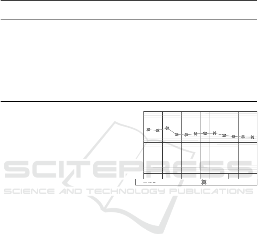
Table 4: Incremental Learning: Overview of TPR scores and relevant meta-features of T at monthly training times t

Time of c

ratio MIS V S

TPR NSF

training M

: 01/2017 97 0.12% 10.90 48.75% 61,21% 5

: 02/2017 124 0.15% 11.64 49.59% 60.92% 9

: 03/2017 152 0.19% 12.48 49.15% 62.00% 22

: 04/2017 188 0.23% 13.48 43.38% 58.80% 19

: 05/2017 222 0.27% 14.47 50.24% 58.74% 1

: 06/2017 272 0.34% 15.47 46.69% 59.26% 12

: 07/2017 320 0.40% 16.47 48.89% 59.46% 24

: 08/2017 379 0.47% 17.47 46.44% 59.50% 18

: 09/2017 440 0.54% 18.47 48.04% 58.55% 5

: 10/2017 488 0.60% 19.47 39.59% 57.92% 17

: 11/2017 554 0.68% 20.47 45.41% 57.90% 3

: 12/2017 640 0.79% 21.47 40.36% 57.88% 2

incremental learning or windowing really address our

DSS and thus lead to improvements in the TPR or not.

5 EVALUATION

We report the results of our experimental study ac-

cording to the setup described in Section 4. First, we

discuss the classiﬁcation results of the two approaches

of incremental learning and windowing in the respec-

tive evaluation scenarios (5.1). Then, we evaluate

data-driven classiﬁers from a domain-speciﬁc point of

view, i. e., the concrete added value for truck manu-

facturers by saving monetary warranty costs (5.2).

5.1 Results for Evaluation Scenarios

Basis for the two approaches of incremental learning

and windowing in the evaluation scenarios is the use

case introduced in Section 2.1. Here, data scientists

train a model early in 2017. So, they use the training

data T with a data status in this year, i. e., the statuses

to t

for the incremental learning approach (see

Table 4). For the evaluation of windowing (Table 5),

we use the ﬁxed data status on 01/01/2017. For the

discussions of the evaluation results, we use the meta-

features c

ratio, MIS and V S

to characterizes

the impacts of the two dataset shifts CS1 and CS2.

Note that we use V S

instead of V S , because our

paramount interest are trucks that will fail in future.

Furthermore, we have listed the best NSF value for

each measurement in both Table 4 and Table 5.

5.1.1 Results for Incremental Learning

Here, we train different classiﬁers monthly with new

labels updated each month (t

1−12

). We then ap-

61.21%

62.00%

58.80%

40%

45%

50%

55%

60%

65%

70%

59.50%

57.92%

57.88%

True-Positive-Rate (TPR)

Baseline (TPR: 55.90%)

Figure 2: Incremental Learning: the y-axis shows the TPR

scores and the x-axis the different points in time t

to t

ply each classiﬁer to the next batch of manufactured

trucks (T

). With the monthly changing data sta-

tuses in 2017, i. e., t

to t

, the expectation is to

start with a less performant model at t

. Neverthe-

less, the more time passes, the better the predictive

performance is supposed to become, since the c

ra-

tio increases monthly. This is because the formation

of current to ﬁnal class patterns converges over time.

Figure 2 shows the TPR scores for each point in

time t

. At time point t

, the TPR is 61.21% and can

even improve to 62% by t

. So, this at ﬁrst glance

corresponds to the expected behavior that the TPR in-

creases over time. However, this expectation is con-

tradicted with following time points, where the TPR

tends to get worse. With 57.88%, the ﬁnal incremen-

tal TPR at the end of the time line (t

) is even lower

than the one at t

. This incremental TPR is signiﬁ-

cantly inﬂuenced by two previous time points: t

and

. The two drops in performance at t

and t

can

be explained by the meta-feature of truck similarity

V S

(see Table 4). On average, the value of V S

is 46.38%, measured from t

to t

. Especially at

ICEIS 2022 - 24th International Conference on Enterprise Information Systems

402

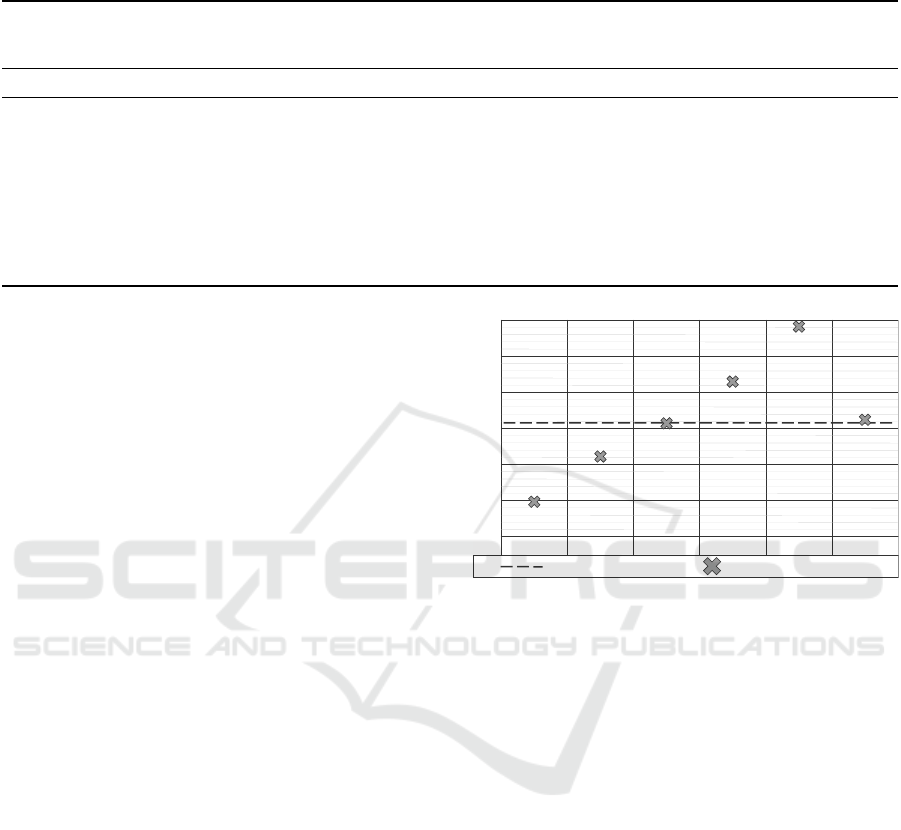
Table 5: Windowing: Overview of TPR scores and relevant meta-features for time-consecutive training subsets (windows) T

The data status for training is always 01/01/2017.

Production c

ratio MIS V S

TPR NSF

window T

T : 2015/16 97 0.12% 10.90 49.95% 55.90% 5

: Q1-2015 9 0.11% 21.35 50.65% 44.83% 17

: Q2-2015 29 0.30% 18.32 52.43% 51.19% 11

: Q3-2015 27 0.26% 15.53 53.89% 55.71% 8

: Q4-2015 17 0.16% 12.40 54.35% 61.51% 4

: Q1-2016 8 0.08% 9.13 60.31% 69.34% 3

: Q2-2016 7 0.06% 6.20 65.11% 56.27% 1

: Q3-2016 0 0.00% 3.17 - - -

: Q4-2016 0 0.00% 0.90 - - -

the time points t

, t

and t

, the V S

values are

however much lower than this average with 43.28%,

39.59% and 40.36%, respectively. Thus, despite in-

creasing c

ratio, the failure behavior represented by

, t

and t

is increasingly different from the fail-

ure behavior of current production batches (T

). We

hence conclude that the covariate shift (CS1) has a

signiﬁcant impact on the poor TPR scores.

The ﬁnal TPR score with incremental learning is

the 57.88% at time point t

. Although this is much

lower than expected, it still constitutes an increase

of 1.98%-points compared to the baseline. Note

that this small improvement may be achieved despite

the above-mentioned negative effects of the covari-

ate shift (CS1). So, incremental learning seems to

address the other dataset shift, i. e., the concept shift

(CS2), at least to a moderate degree. This is also evi-

dent, as the c

ratio increases monthly (see Table 4).

Altogether, the behavior of the incremental TPR

and our discussion above prove the non-trivial trade-

off relationship between CS1 and CS2 and that it

constitutes a challenge for approaches to incremental

learning. In the following, we investigate this trade-

off in more detail via the approach of windowing.

5.1.2 Results for Windowing

Here, we split the dataset T into eight training subsets

1−8

). Since the subsets T

7−8

do not contain failed

trucks, we can only train classiﬁers with the subsets

1−6

, respectively the windows (T

). We then apply

each trained classiﬁer on all trucks in T

and measure

the resulting TPR scores for each window T

Figure 3 shows the TPR scores for each window

. For windows T

to T

, it is noticeable that the

TPR scores get better with each window and thus with

decreasing truck age. This is due to the fact that al-

though the c

ratio is higher in the ﬁrst windows, the

lack of similarity leads to a weaker predictive perfor-

40%

True-Positive-Rate (TPR)

Baseline (TPR: 55.90%)

45%

50%

55%

60%

65%

70%

44.83%

51.19%

55.71%

61.51%

69.34%

56.27%

Figure 3: Windowing: the y-axis shows the TPR scores and

the x-axis the different windows T

to T

mance (TPR). Thus, older trucks in T

are less similar

to the failed trucks in T

than newer trucks from T

Going further with the subsequent window T

, the

TPR value decreases by about 13%-points although

the V S

value is higher than at T

. This drop in

performance can be explained by the decrease in c

ratio due to the low average MIS of the trucks in

. Among all subsets, the covariate shift (CS1) has

the lowest negative impact on the TPR at T

(V S

65.11%), because these trucks are most similar to the

current production. This is contrasted by the concept

shift (CS2), which has the highest negative impact on

the TPR at T

ratio: 0.06%), among all subsets.

Moving from subset T

to the left, the negative ef-

fect of CS2 decreases by the fact that the trucks have

already been in use for a longer time. So, they had

a higher chance to fail and the c

ratio is usually

higher for subsets with older trucks. However, it is

evident from the V S

values in Table 5 that older

failed trucks in early subsets T

are less similar to the

failed trucks in the test set T

. So, an higher average

age of trucks leads to an increase in the negative ef-

fects of CS1. Summarized, both dataset shifts have

Analysis of Incremental Learning and Windowing to Handle Combined Dataset Shifts on Binary Classiﬁcation for Product Failure

Prediction

403

negative impacts on the True-Positive-Rate. Thus, we

cannot state which dataset shift is more dominant.

Only the training of classiﬁers on subsets T

and

leads to an increase of the TPR compared to the

baseline. Training the classiﬁer on T

leads to an in-

crease of the TPR by 5.61%-points, whereas training

on T

leads to an increase of 13.44%-points. The win-

dow T

represents the most balanced dataset, as both

ratio and truck similarity V S

have high val-

ues (see Table 5). Trucks in T

are old enough (MIS:

9.13) to have an adequate number of failures (c

ra-

tio: 0.08%), and those failed trucks have a adequate

similarity (V S

: 65.11%) to the failed trucks in T

5.2 Domain-speciﬁc Evaluation

Now we discuss the concrete added value that data-

driven classiﬁers imply in terms of saving monetary

warranty costs. In this context, we compare the po-

tentials of cost savings yielded by the employed ap-

proaches to incremental learning and windowing with

the baseline. This baseline is a classiﬁer trained on the

entire training dataset T without explicitly addressing

the two dataset shifts and results in a TPR of 55.9%.

In order to highlight the potential cost savings in

practical use, we assume that each repair of the partic-

ular damage leads to warranty costs of about $2,500.

Note that this is a conservative assumption because

the scope of components that may fail is very wide.

Corresponding to the 4,585 failed trucks in T

, this

results in a total of ∼ $11.4 million in warranty costs.

The ﬁnal TPR achieved by the approach to incre-

mental learning is 57.88%. So, it can reduce the fail-

ure rate by 1.98%-points compared to the TPR of the

baseline. With 4,585 failed trucks contained in T

(see Table 2), this leads to about 91 less truck fail-

ures. It hence results in potential cost savings of about

$0.2 million. The cost savings yielded by windowing

are however much higher. Here, the best TPR score

of 69.34% is achievable with the training subset T

resulting in a reduction of the failure rate by 13.44%-

points. So, we may prevent with windowing 616 more

failures, resulting in potential cost savings of approxi-

mately $1.5 million. This is a signiﬁcant reduction of

avoidable warranty claims and consequential costs.

The experimental analyses show that the best clas-

siﬁer to deal with combined DSS is trained with the

Random Forest algorithm, NSF sampling, quarter-

wise windowing, and grid search hyperparameter op-

timization. In practice, it is however difﬁcult and

complex to ﬁnd the best training subset, i. e., T

. This

is due to the fact that a ﬁnal TPR score can only be

measured after waiting a period of several years or at

least the warranty period of the future trucks. There-

fore, further research is needed to devise approaches

that may early identify those windows yielding a high

predictive performance of the classiﬁer without wait-

ing that long period of time. In contrast, incremental

learning can directly be applied and save $0.2 million.

6 CONCLUSION AND FUTURE

WORK

In this paper, we discuss our experimental study for

a real-world use case of a data-driven prediction of

product failures. We provide insights into the data

characteristics in such real-world scenarios and into

two kinds of dataset shifts (DSS) that result from

these data characteristics: a covariate shift (CS1) and

a concept shift (CS2). In contrast to the assump-

tions made in literature, these two kinds of dataset

shifts usually occur together in real-world use cases.

Furthermore, both DSS show a trade-off relationship,

i. e., choosing data to avoid one, risks making the

other one worse. With our experimental study, we

prove that existing approaches to addressing DSS,

e. g., incremental learning and windowing especially

struggle with this trade-off relationship between CS1

and CS2. Nevertheless, our evaluation shows that

both approaches may still be used to train classiﬁers

that yield better results than the baseline of a classiﬁer

that does not address DSS at all. For instance, the use

of incremental learning leads to a True-Positive-Rate

(TPR) of 57.88%. This still outperforms the baseline

by 1.98%-points. Although these TPR scores are low

from a data science perspective, this has the potential

to realize monetary cost savings for manufacturers.

In future, we are going to develop novel ap-

proaches to pre-process the data in order to ade-

quately address both covariate shift (CS1) and con-

cept shift (CS2). For instance, a domain-speciﬁc

sampling strategy may incorporate the meta-features

V S

and MIS to select only trucks for the training

dataset that are less affected by the two dataset shifts.

ACKNOWLEDGEMENTS

The authors thank the German Research Foundation

(DFG) and the Ministry of Science, Research and Arts

of the State of Baden-Wurttemberg for ﬁnancial sup-

port of this work within the Graduate School of Ex-

cellence advanced Manufacturing Engineering.

ICEIS 2022 - 24th International Conference on Enterprise Information Systems

404

REFERENCES

Bang, S. H., Ak, R., Narayanan, A., Lee, Y. T., and Cho,

H. (2019). A survey on knowledge transfer for man-

ufacturing data analytics. Computers in Industry,

104:116–130.

Bifet, A. and Gavald

a, R. (2007). Learning from time-

changing data with adaptive windowing. In Proceed-

ings of the 2007 SDM.

Boiko Ferreira, L. E., Murilo Gomes, H., Bifet, A., and

Oliveira, L. S. (2019). Adaptive random forests with

resampling for imbalanced data streams. In 2019

IJCNN, pages 1–6.

Bordes, A., Ertekin, S., Weston, J., and Bottou, L. (2005).

Fast kernel classiﬁers with online and active learning.

Journal of Machine Learning Research, 6:1579–1619.

Breiman, L. (1996). Bagging predictors. Machine Learn-

ing, 24(2):123–140.

Breiman, L. (2001). Random forests. Machine Learning,

45(1):5–32.

Cortes, C. and Vapnik, V. (1995). Support-vector networks.

Machine learning, 20(3):273–297.

Degenhardt, F., Seifert, S., and Szymczak, S. (2017). Evalu-

ation of variable selection methods for random forests

and omics data sets. Brieﬁngs in bioinformatics, 20.

Dharani Y., G., Nair, N. G., Satpathy, P., and Christopher,

J. (2019). Covariate shift: A review and analysis on

classiﬁers. In 2019 GCAT, pages 1–6.

Ditzler, G., Roveri, M., Alippi, C., and Polikar, R. (2015).

Learning in nonstationary environments: A survey.

IEEE CIM, 10(4):12–25.

Domingos, P. and Hulten, G. (2002). Mining high-speed

data streams. Proceeding of the Sixth ACM SIGKDD.

Ducange, P., Marcelloni, F., and Pecori, R. (2021). Fuzzy

hoeffding decision tree for data stream classiﬁcation.

Int. Journal of Comput. Intell. Systems, 14(1):946.

Elwell, R. and Polikar, R. (2011). Incremental learning

of concept drift in nonstationary environments. IEEE

Transactions on Neural Networks, 22(10):1517–1531.

Gomes, H. M., Bifet, A., Read, J., Barddal, J. P., En-

embreck, F., Pfharinger, B., Holmes, G., and Ab-

dessalem, T. (2017). Adaptive random forests for

evolving data stream classiﬁcation. Machine Learn-

ing, 106(9-10):1469–1495.

Gunduz, N. and Fokoue, E. (2015). Robust classiﬁca-

tion of high dimension low sample size data. arXiv:

1501.00592.

Hasanin, T., Khoshgoftaar, T. M., Leevy, J., and Seliya,

N. (2019). Investigating random undersampling and

feature selection on bioinformatics big data. In 2019

IEEE BigDataService, pages 346–356.

Hirsch, V., Reimann, P., and Mitschang, B. (2019). Data-

driven fault diagnosis in end-of-line testing of com-

plex products. In 2019 IEEE DSAA, pages 492–503.

Homayoun, S. and Ahmadzadeh, M. (2016). A review on

data stream classiﬁcation approaches. Journal of Ad-

vanced Computer Science & Technology, 5(1):8.

Iwashita, A. S. and Papa, J. P. (2019). An overview on con-

cept drift learning. IEEE Access, 7:1532–1547.

John, G. H., Kohavi, R., and Pﬂeger, K. (1994). Irrelevant

features and the subset selection problem. In Cohen,

W. W. and Hirsh, H., editors, Machine Learning Pro-

ceedings 1994, pages 121–129. Morgan Kaufmann,

San Francisco (CA).

Khan, A. and Usman, M. (2015). Early diagnosis of

alzheimer’s disease using machine learning tech-

niques: A review paper. In 2015 IC3K, volume 01,

pages 380–387.

Khoshkangini, R., Pashami, S., and Nowaczyk, S. (2019).

Warranty claim rate prediction using logged vehicle

data. In Moura Oliveira, P., Novais, P., and Reis, L. P.,

editors, Progress in AI, pages 663–674.

Kull, M. and Flach, P. (2014). Patterns of dataset shift.

First International Workshop on Learning over Mul-

tiple Contexts (LMCE) at ECML-PKDD.

Losing, V., Hammer, B., and Wersing, H. (2018). Incremen-

tal on-line learning: A review and comparison of state

of the art algorithms. Neurocomputing, 275:1261–

1274.

Lu, J., Liu, A., Dong, F., Gu, F., Gama, J., and Zhang,

G. (2019). Learning under concept drift: A review.

IEEE Transactions on Knowledge and Data Engineer-

ing, 31(12):2346–2363.

Mait

ın, A. M., Garc

ıa-Tejedor, A. J., and Mu

noz, J. P. R.

(2020). Machine learning approaches for detecting

parkinson’s disease from eeg analysis: A systematic

review. Applied Sciences, 10(23).

Marron, J., Todd, M., and Ahn, J. (2007). Distance-

weighted discrimination. Journal of the American Sta-

tistical Association, 102:1267–1271.

Moreno-Torres, J. G., Raeder, T., Alaiz-Rodr

ıguez, R.,

Chawla, N. V., and Herrera, F. (2012). A unifying

view on dataset shift in classiﬁcation. Pattern Recog-

nition, 45(1):521–530.

Nalbach, O., Linn, C., Derouet, M., and Werth, D. (2018).

Predictive quality: Towards a new understanding of

quality assurance using machine learning tools. In

Business Information Systems, pages 30–42. Springer

International Publishing.

Pearson, K. (1901). LIII. on lines and planes of closest ﬁt to

systems of points in space. The London, Edinburgh,

and Dublin Philosophical Magazine and Journal of

Science, 2(11):559–572.

Prytz, R., Nowaczyk, S., R

ognvaldsson, T., and Byttner, S.

(2015). Predicting the need for vehicle compressor

repairs using maintenance records and logged vehi-

cle data. Engineering Applications of Artiﬁcial Intel-

ligence, 41:139–150.

Qui

nonero-Candela, J., Sugiyama, M., Schwaighofer, A.,

and Lawrence, N. D., editors (2008). Dataset Shift in

Machine Learning. The MIT Press.

Turki, T. and Wei, Z. (2016). A greedy-based oversam-

pling approach to improve the prediction of mortality

in mers patients. In 2016 Annual IEEE Systems Con-

ference (SysCon), pages 1–5.

Utgoff, P. E. (1989). Incremental induction of decision

trees. Machine Learning, 4(2):161–186.

Wu, S. (2013). A review on coarse warranty data and anal-

ysis. Reliability Eng. & System Safety, 114:1–11.

Analysis of Incremental Learning and Windowing to Handle Combined Dataset Shifts on Binary Classiﬁcation for Product Failure

Prediction

405