Increasing Explainability of Clustering Results for Domain Experts by

Identifying Meaningful Features

Michael Behringer

, Pascal Hirmer

, Dennis Tschechlov and Bernhard Mitschang

Institute of Parallel and Distributed Systems, University of Stuttgart, Universit

atsstr. 38, 70569 Stuttgart, Germany

Keywords:

Clustering, Explainability, Human-in-the-Loop.

Abstract:

Today, the amount of data is growing rapidly, which makes it nearly impossible for human analysts to com-

prehend the data or to extract any knowledge from it. To cope with this, as part of the knowledge discovery

process, many different data mining and machine learning techniques were developed in the past. A famous

representative of such techniques is clustering, which allows the identiﬁcation of different groups of data (the

clusters) based on data characteristics. These algorithms need no prior knowledge or conﬁguration, which

makes them easy to use, but interpreting and explaining the results can become very difﬁcult for domain ex-

perts. Even though different kinds of visualizations for clustering results exist, they do not offer enough details

for explaining how the algorithms reached their results. In this paper, we propose a new approach to increase

explainability for clustering algorithms. Our approach identiﬁes and selects features that are most meaningful

for the clustering result. We conducted a comprehensive evaluation in which, based on 216 synthetic datasets,

we ﬁrst examined various dispersion metrics regarding their suitability to identify meaningful features and we

evaluated the achieved precision with respect to different data characteristics. This evaluation shows, that our

approach outperforms existing algorithms in 93 percent of the examined datasets.

1 INTRODUCTION

Nowadays, a tremendous amount of data is being cap-

tured, stored, and processed throughout almost any

domain. With the progressing digitalization, this data

keeps growing every day. Analyzing this data leads to

new possibilities for improving our daily lives, e. g.,

through automated trafﬁc management or easier di-

agnosis of illnesses. However, for a domain expert,

oftentimes the amount of data is too large to be com-

prehended, processed, or analyzed (Keim et al., 2008;

Maimon and Rokach, 2010). For this reason, many

techniques exist for data mining and machine learn-

ing with the goal of extracting information and knowl-

edge from data. This is referred to as the knowledge

discovery process (Fayyad et al., 1996). A popular

data mining technique is clustering (Wu et al., 2008),

which assigns similar data to a cluster based on the

data’s characteristics. This allows identifying clus-

ters in the data without any speciﬁc prior knowledge.

A famous and widely used representative for these al-

gorithms is k-Means (MacQueen, 1967).

https://orcid.org/0000-0002-0410-5307

https://orcid.org/0000-0002-2656-0095

However, when it comes to clustering, interpreting

and explaining the results can become difﬁcult. Since

there is no prior knowledge of the data, it can become

unclear how the algorithms created the clusters, i. e.,

which data characteristics were relevant or how the

data of different clusters can even be distinguished.

Being able to comprehend and explain the results,

however, is an important issue for domain experts,

since they can only trust in the results if they are able

to understand how they were concluded. Hence it is

necessary to keep the human user ”in-the-loop” (En-

dert et al., 2014; Behringer et al., 2017).

To cope with the issue of data interpretation, dif-

ferent preparation and visualization techniques were

developed for clustering, e. g., Principal Component

Analysis (PCA) (Dunteman, 1989) or t-Distributed

Stochastic Neighbor Embedding (t-SNE) (Hinton and

Roweis, 2002). When applying PCA to a multi-

dimensional dataset, the dataset is reduced to fewer

dimensions while preserving as much of the data’s

characteristics as possible and in order to increase

comprehensibility. In contrast, t-SNE is a non-linear

dimension reduction technique that creates a visual

result in two or three dimensions to evaluate segmen-

tation for exploration purposes.

364

Behringer, M., Hirmer, P., Tschechlov, D. and Mitschang, B.

Increasing Explainability of Clustering Results for Domain Experts by Identifying Meaningful Features.

DOI: 10.5220/0011092000003179

In Proceedings of the 24th International Conference on Enterprise Information Systems (ICEIS 2022) - Volume 2, pages 364-373

ISBN: 978-989-758-569-2; ISSN: 2184-4992

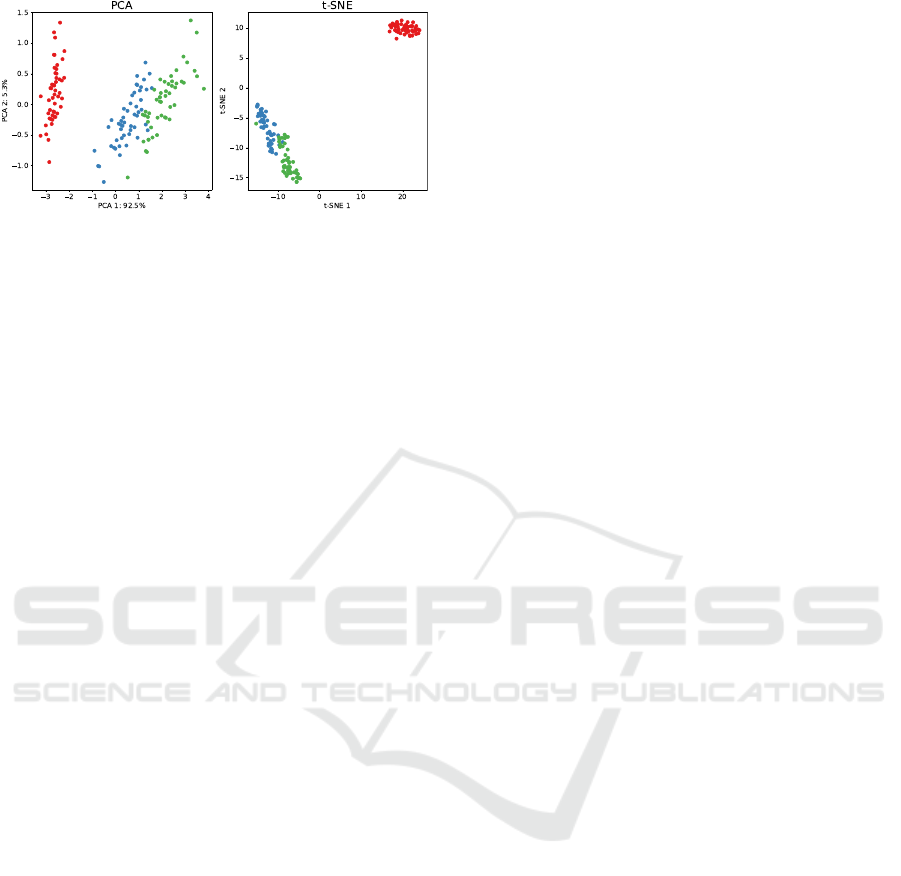
Figure 1: The results of PCA and t-SNE on the IRIS dataset.

Figure 1 shows the visualization results based on

PCA and t-SNE on the IRIS dataset (Fisher, 1988). In

PCA, ﬁnding clusters can be difﬁcult, depending on

the number of clusters and data distribution. In the

example on the right, using t-SNE, although clusters

can be identiﬁed easily, details of the data are lacking,

however, since the concrete range of values in the data

as well as the semantics of the axes cannot be seen at

glance by human users.

In addition to PCA or t-SNE, data mining tools

like WEKA (Frank et al., 2016) offer a textual repre-

sentation of clustering results, which contains many

details about how the clustering result was reached,

e. g., the number of necessary iterations, statistical in-

dicators like mean or standard deviation, or the num-

ber of instances per cluster. Experienced data sci-

entists can draw conclusions from this kind of infor-

mation, however, there is no ﬁltering for relevant in-

formation. In particular, considering results with an

increasing number of features, it becomes more and

more difﬁcult to maintain an overview, and human

analysts can easily become overwhelmed by such tex-

tual representations.

In many cases, however, it is purposeful if anal-

yses are not performed by dedicated data scientists,

but to enable domain experts to perform these anal-

yses themselves, e.g., for accelerated initial results.

This is referred to as self-service business intelli-

gence (Imhoff and White, 2011). Hence, using state-

of-the-art approaches still makes explaining how the

algorithms reached their results a great challenge.

To cope with this issue, we introduce in this paper

a new approach to enhance the explainability of clus-

tering algorithms. In the ﬁrst step, we create a rank-

ing of features by the meaningfulness for the result

of the clustering algorithm. Subsequently, we deter-

mine the quantity of features that are to be considered

meaningful in order not to overwhelm a domain ex-

pert. Next, we calculate statistical parameters, which

reduce the amount of information, leading to an eas-

ier understanding and further insights. These param-

eters, e. g., minimum, maximum or upper and lower

quartile, are calculated for each selected feature.

For the purpose of evaluation, we compare our ap-

proach against a state-of-the-art approach based on

216 synthetic datasets with a wide range of different

characteristics and show that our approach offers sig-

niﬁcant advantages and, in terms of identiﬁed mean-

ingful features, outperforms the state-of-the-art ap-

proach in up to 93 percent of the datasets.

The remainder of this paper is structured as fol-

lows: Section 2 introduces related work. Next, Sec-

tion 3 contains our main contribution – an approach to

increase explainability of clustering algorithms. Sec-

tion 4 shows the results of our evaluation. Finally,

Section 5 concludes this paper.

2 RELATED WORK

Clustering is an unsupervised data mining technique

to discover groups in the given dataset, such that

the data within a cluster are similar and the data

of different clusters are dissimilar. In the litera-

ture, several clustering algorithms exist (Jain, 2010).

The most famous ones are centroid-based, such as

k-Means (MacQueen, 1967), density-based, such as

DBSCAN or OPTICS (Ester et al., 1996), and hier-

archical ones (Jain, 2010). Here, k-Means is a very

famous clustering algorithm due to its ease of use and

scalability (Wu et al., 2008). However, all these clus-

tering algorithms require parameters to be set prior to

execution. Yet, the parameters highly inﬂuence the

clustering result. For instance, centroid-based algo-

rithms such as k-Means require the number of clusters

as input.

To detect the number of clusters, automatic and

semi-automatic methods exist in the literature. Both

ﬁrst execute a clustering algorithm with several possi-

ble values for the parameters, e. g., for the number of

clusters on the dataset. Automatic methods use clus-

tering metrics to evaluate the clustering results and to

choose the best one automatically (Liu et al., 2013).

There are actually two kinds of clustering metrics:

External and internal metrics. External metrics com-

pare the clustering result against a ground-truth clus-

tering result. However, in general, we cannot assume

that we have information about the ground truth as

clustering is a solely unsupervised task. In contrast,

internal metrics measure the compactness (similarity

between instances within one cluster) and dispersion

(dissimilarity between different clusters) of cluster-

ing results and set both measures in relation to each

other. Here, various metrics exist, e. g., the Silhou-

ette (Rousseeuw, 1987), Davies-Bouldin (Davies and

Bouldin, 1979) or Calinski-Harabasz (Cali

nski and

Harabasz, 1974).

Increasing Explainability of Clustering Results for Domain Experts by Identifying Meaningful Features

365

A prevalent semi-automatic method is the elbow

method (Thorndike, 1953). The user is shown a graph

over the different k values on the x-axis and the y-axis

shows the sum of square errors for the corresponding

k value. This graph is typically monotonic decreas-

ing, however, the assumption here is that the correct k

value is the one with the highest decrease. This point

of the highest decrease can be obtained by looking

at the graph and searching for an elbow point by the

user. Yet, the automatic and semi-automatic methods

can only compare different clustering results and tell

which one is better, but cannot describe how a clus-

tering result is obtained and which are the meaningful

features that led to each individual cluster.

To detect the most signiﬁcant features in data, fea-

ture selection (Kumar and Minz, 2014) or feature im-

portance (Altmann et al., 2010) algorithms might be

used. The most common use of feature selection is

that based on a target class, e. g., the cluster label, the

features that have the greatest impact on the result are

selected. These algorithms typically assign scores to

the features by measuring the correlation of a feature

with respect to the target. To this end, statistical mea-

sures as, for instance, ANOVA, chi-square or mutual

information are used (Altmann et al., 2010).

Yet, there are also more advanced feature selection

algorithms, e. g., Random Forest (Breiman, 2001) or

Boruta (Kursa and Rudnicki, 2010), which uses a

Random Forest model to predict which features con-

tribute most to the result. However, it is not possible

to apply these algorithms on the resulting clusters in-

dividually as each cluster contains only one label and

thus meaningful statements are not possible if only

one class is present. Hence, these approaches are not

suited to explain which features are important in the

individual clusters or the clustering result at all.

However, some feature selection algorithms can

be used without a target class (Solorio-Fern

andez

et al., 2020). Here, the authors conclude that addi-

tional hyperparameters, such as the number of clus-

ters or number of features, are needed for such fea-

ture selection algorithms, which are not available in

practice by domain experts, especially in the context

of exploratory analysis. Furthermore, the scalability

of these methods is limited and differences between

individual clusters and the entire dataset are not taken

into account. As a result, meaningful features can not

be determined for each cluster individually.

The most related approach to our work is Inter-

pretable k-Means (Alghofaili, 2021) which yet is not

a scientiﬁc publication but a promising article pub-

lished on towardsdatascience.com including imple-

mentation on GitHub. This approach utilizes the SSE

that is minimized in the k-Means method. To this end,

it calculates for each cluster which feature minimized

the SSE the most. Since the objective of k-Means is

to minimize the SSE, this would relate to the feature

with the most signiﬁcant impact to the clustering re-

sult. This allows to assign a feature importance score

to each feature and to select the most meaningful fea-

tures on this basis. Though this method is able to se-

lect features for each cluster individually, it is only

applicable to k-Means.

Approaches that aim to increase the explainability

and the interpretation of clustering results typically

use decision trees (Dasgupta et al., 2020; Loyola-

Gonz

alez et al., 2020) for that purpose. Though, de-

cision trees are supervised methods, they can be used

on the clustering result by using the cluster labels as

class labels. Then, a decision tree is trained on the

clustering results. The resulting decision tree can sub-

sequently be used to explain for a certain data instance

why it belongs to a cluster. Though this is suitable to

explain why certain instances are within a cluster, this

is not suitable for domain experts if there are thou-

sands or millions of data instances. As a consequence,

explaining every single instance is not scalable for do-

main experts and it remains uncertain by what one

cluster is characterized in detail. Hence, we follow

a different approach, i. e., we aim to summarize and

describe the clusters themselves and not each data in-

stance. Therefore, our approach is especially more

suited for large-scale datasets where we might have

millions of data instances with hundreds of features.

With regard to commercial software, there is an

option in IBM DB2 Warehouse to visualize and com-

municate clustering results. Thereby exists the oppor-

tunity to sort the features according to their impor-

tance. However, based on the documentation

, this

sorting contains all features and is based either on the

normalized chi-square values, the homogeneity of the

values, or in alphabetical order.

In summary, approaches to explain clustering re-

sults only describe the generation, e.g., by decision

trees, but not the content or meaning of the result.

Feature selection algorithms can only be used to iden-

tify meaningful features for the entire result, but not

for individual clusters. The only algorithm we could

ﬁnd for identifying meaningful features at the clus-

ter level, Interpretable k-Means, is limited to k-Means

and thus not generally applicable. Furthermore, Inter-

pretable k-Means a) ignores the differences between

clusters and the entire dataset and b) lacks function-

ality to determine the quantity of meaningful features

and instead returns a ranking over all features avail-

able in the dataset.

https://www.ibm.com/docs/en/db2/10.5

ICEIS 2022 - 24th International Conference on Enterprise Information Systems

366

3 EXPLAINABILITY OF

CLUSTERING RESULTS USING

MEANINGFUL FEATURES

Clustering aims at combining similar data into

groups. This is done by maximizing separation be-

tween the clusters and minimizing separation within

a cluster. To determine this degree of separation,

metrics are used, such as the distance between the

points (k-Means), the distance between the neighbor-

ing points (DBSCAN), or the graph distance (e. g., the

nearest-neighbor graph on spectral clustering). Ac-

cordingly, a good clustering result is achieved when

instances from different clusters differ strongly, i. e.,

the dispersion is rather large, while the dispersion

within a cluster is small. However, a clustering re-

sult considered as optimal based on objective criteria,

such as dispersion or compactness metrics, is not nec-

essarily appropriate in each scenario. Instead, non-

optimal clustering results may be more expressive and

provide more value to an analysis given that they bet-

ter represent the real world. Hence, an interpretation

purely on these metrics is difﬁcult for domain experts.

In particular, large datasets contain many features

that are not relevant for the clustering result but make

interpretation of the result an even more difﬁcult task.

In order to interpret a clustering result, it is therefore

crucial that the features that are most meaningful are

identiﬁed and subsequently processed in a way that

can easily be interpreted by domain experts.

To accomplish this, four steps are necessary:

(1) identiﬁcation of meaningful features, (2) deter-

mine the quantity of meaningful features, (3) determi-

nation of statistical quantities, and (4) visualization of

the results:

(1) Identiﬁcation of Meaningful Features. For the

ﬁrst step, we assume that dispersion metrics are not

only suitable for assessing the overall result, but also

for analyzing individual features in isolation. Conse-

quently, a feature is considered meaningful as long as

the dispersion of this feature within a cluster is clearly

different from the dispersion of this feature in the en-

tire dataset. In order to ﬁnd the meaningful features,

we calculate for each cluster c

and feature f

an arbi-

trary metric M, for instance, the variance or standard

deviation.

In Sect. 4, we examine a selection of different dis-

persion metrics for their suitability with respect to this

application. Subsequently, we calculate this metric

for the feature f

as well on the entire dataset to get

the metric difference:

MetricDi f f erence

, f

= |M

, f

| − |M

all

, f

| (1)

This metric difference (cf. Eq. 1) is minimized when

the dispersion of values of the considered feature f

within the considered cluster c

is small (|M

, f

|) and

the dispersion over all clusters c

all

, i. e., the entire

dataset, is large for this feature (|M

all

, f

|). The metric

difference can now be used to identify the most mean-

ingful features for each single cluster individually and

to rank the features for each cluster. Note, that each

feature has to be normalized to ensure comparability

between features. Nevertheless, it may be relevant for

a domain expert to identify the most meaningful fea-

tures across all clusters. For this purpose, for each

feature, the position in the respective cluster ranking

can be leveraged and the features with the best av-

erage position are identiﬁed as the most meaningful

features across all clusters.

In some cases, however, depending on the speciﬁc

analysis scenario it is more appropriate to understand

why clusters are separated. Hence, the most meaning-

ful features are those that make clusters most distin-

guishable from one another, even if these features do

not describe the cluster itself anymore. If so, it is not

the dispersion between feature and entire dataset that

has to be considered, but the discriminatory power

(DP, cf. Eq.2) of the value ranges for a feature be-

tween the different clusters:

= (MO

, ID

) (2)

Thus, for each feature f

of the dataset, there is one

tuple composed by the degree of the mean overlap

(MO

, cf. Eq. 3) as well as the inner distance (ID

cf. Eq. 5). Both are discussed in more detail below.

c ∗ (c − 1)

∑

i=1

∑

j=1

j6=i

, c

)

max

) − min

)

(3)

, c

) = max(0, min(max

), max

))

− max(min

), min

)))

(4)

First, the average degree of overlap (MO

) is cal-

culated. This describes the pairwise overlap (O

cf. Eq. 4) of the value ranges between the currently

considered cluster c

and all other clusters c

for the

feature f

. This overlap is also set in relation to the

respective value range covered, i.e, if the currently

considered cluster c

covers a larger value range, then

an overlap of the same size is less penalizing than in

the case of a smaller value range. Consequently, a

result in which the value ranges of a feature do not

overlap between different clusters is in general bet-

ter than one with overlap, but it is rather unlikely to

achieve this kind of accurate separation. It is more

likely that the same overlap will occur between two

Increasing Explainability of Clustering Results for Domain Experts by Identifying Meaningful Features

367

different features. If this happens, the feature that sep-

arates the value ranges more strongly should be con-

sidered as more meaningful, i. e., the so-called inner

distance (ID

, cf. Eq. 5) between the value ranges

of the clusters is larger. This inner distance is larger

when less value range is occupied by different clus-

ters at the same time. It should be noted that the use

of minimum and maximum is quite susceptible to out-

liers. To reduce this risk, the interquartile range could

be used instead of minimum and maximum, however,

it has to be accepted that the results may be altered in

this scenario.

= 1 −

∑

i=1

max

) − min

)

(5)

Based on the introduced metric difference, it is

possible to identify the meaningful features for each

cluster both individually and over the entire group

of clusters. Furthermore, by considering the value

ranges in the discriminatory power DP, it is also fea-

sible to identify the features that distinguish the clus-

ters most signiﬁcantly. Thus, we are able to identify

meaningful features for each single cluster, for an en-

tire clustering result across clusters and, ﬁnally, dis-

tinguishing clusters from each other. This step ends

with a ranking of the features based on their mean-

ingfulness.

(2) Determine the Quantity of Meaningful Fea-

tures. In the second step, it must be decided, based on

the ranking of the features, which features are mean-

ingful and enable a domain expert to interpret the

clustering result. Here, three different approaches can

be considered:

(a) Static. Humans can only process a small

amount of information, which is why a focus on the

relevant information is required. According to stud-

ies (Miller, 1956), about 5-9 different values are fea-

sible simultaneously. For the sake of perception, the

number of features can be set to a ﬁxed number, e. g.,

the lower limit 5, and accordingly, the top 5 of the

most meaningful features will be selected as mean-

ingful. This guarantees perceptibility, but if less than

these 5 features are actually meaningful, the selection

would still be increased to 5 features and the domain

expert might draw wrong conclusions.

(b) Threshold. As an alternative, a ﬁxed threshold

for the results from step 1 could be set, which is either

pre-conﬁgured or can be changed by the domain ex-

pert during the analysis. After setting this threshold,

all features that fall below it are selected. However, if

the threshold is set too high, it means that too many

features are selected and the results are difﬁcult for a

domain expert to interpret. Instead, if the threshold is

set too low, it is possible that no features are selected

at all as long as no feature falls below this threshold.

However, setting this threshold properly depends on

the data and is, therefore, not reliable in all cases, as

domain experts tend to set it in a way that their expec-

tations are fulﬁlled even if the features are not mean-

ingful at all (bias).

popular Elbow Method (cf. Sect. 3.2), which is com-

monly used to determine the correct number of clus-

ters and use it to identify the quantity of meaningful

features. To do this, the features are sorted accord-

ing to the calculated metric value, which is given here

in advance due to step 1. Subsequently, for each pair

of adjacent features in the ranking, it is determined

how large the change between these features is. If a

large change (knick/elbow) occurs, this means that the

meaningfulness between these features has changed

signiﬁcantly. In this way, it can be decided in a dy-

namic way which features are still considered mean-

ingful and which are no longer meaningful. In order

to avoid that too many features are considered mean-

ingful, in case of small changes between the features,

the number of features can be as limited as in the static

approach. In contrast to the static approach, however,

it is ensured here that no mixture between meaningful

and non-meaningful features is taken into account.

(3) Calculation of Statistical Quantities. The mean-

ingful features are useful on their own but the discrim-

inatory power is still difﬁcult for a domain expert to

interpret. For this reason, for each feature identiﬁed as

meaningful, statistical metrics still need to be calcu-

lated. In the simplest case, it is sufﬁcient to use mini-

mum and maximum values, since overlapping ranges

of values can already be identiﬁed using these values.

However, more complex indicators such as quantiles,

among others, are also conceivable.

(4) Visualizing the Results. Finally, the identiﬁed

meaningful features must be presented to the domain

expert. Here, a large selection from the above options

is available. Of course, a domain expert must ﬁrst se-

lect the algorithm and the corresponding parameters.

Then it has to be decided what should be explained,

i. e., whether the meaningful features should be iden-

tiﬁed for each cluster individually, for the entire clus-

tering result, or the distinction between the individual

clusters. Furthermore, it has to be decided which of

the methods should be used to determine the quantity.

Finally, various visualization techniques exist that can

provide further insights, e. g., histograms and parallel

coordinates plots.

ICEIS 2022 - 24th International Conference on Enterprise Information Systems

368

4 EVALUATION

In order to verify the practicability of our introduced

approach, we have conducted a comprehensive eval-

uation on the basis of synthetic datasets with varying

dataset characteristics, e. g., the number of features or

number of instances. Therefore, we compare multi-

ple dispersion metrics, which are used to calculate the

metric difference in step 1 of our approach and serve

as a basis for the identiﬁcation of meaningful features.

Subsequently, we evaluate the precision achieved in

identifying meaningful features based on the identi-

ﬁed metric.

4.1 Dataset Generation

For the evaluation of the presented approach, we

use synthetic datasets with varying characteristics to

cover a wide range of scenarios, which contain a

ground truth about the contained meaningful features.

To provide this ground truth, 5 features were deﬁned

as meaningful for each dataset, i. e., the values as-

signed to these features follow a normal distribution

within each cluster. A normal distribution is appro-

priate because many real-world measurements follow

this distribution as well. For the non-meaningful fea-

tures, in contrast, a uniform distribution of values was

chosen. This leads to a simulated clustering result

with 5 meaningful features and a varying amount of

non-meaningful features. Note that all features are

generated using the same value range, i. e., the data

is already normalized. The general procedure for c

clusters, n instances, f features and a noise ratio r

between 0 and 1 is as follows: Generate c empty clus-

ters, (2) add

instances with meaningful and non-

meaningful features to each cluster, (3) create n ∗ r

additional instances (noise) with random feature val-

ues, (4) cluster the resulting dataset into the given c

clusters using k-Means++.

Table 1: Overview of the parameters used for the dataset

generation. Each possible permutation was used once.

Parameter Small Datasets Large Datasets

#features f 10, 20, 40 25, 50, 100

#instances n 5.000, 10.000, 50.000 100.000, 500.000, 1.000.000

#clusters c 5, 10, 25 10, 25, 50

noise ratio r 0.00, 0.33, 0.66, 0.99 0.00, 0.33, 0.66, 0.99

In order to cover a broad spectrum of different

dataset characteristics, we generate a large number

of different datasets (in total 216 varying datasets)

using the above-mentioned procedure. Furthermore,

we divide the generated datasets into large and small

datasets to identify potential differences in relation to

the dataset size. Table 1 shows the different parame-

ters we used to create the evaluation datasets. Thus,

every possible combination of these parameters is the

dataset characteristic of exactly one dataset. As a re-

sult, we generate 108 small and 108 large datasets as

the basis for the evaluation and, for each dataset, the

meaningful and purely random features are known.

4.2 Results

The results of our evaluation are divided into two

parts. First, different dispersion metrics are bench-

marked with respect to their performance to identify

meaningful features. Subsequently, a more detailed

evaluation is performed for the most suitable metric

with respect to different dataset characteristics.

4.2.1 Comparison of Dispersion Metrics

Since the identiﬁcation of meaningful features is

based on dispersion metrics, the ﬁrst step is to check

which dispersion metric is best suited to calculate the

metric difference (cf. Eq. 1). Therefore, for each clus-

ter it was ﬁrst calculated how many of the original 5

meaningful features are found in the top 5 features of

this cluster, e. g., if 3 of 5 meaningful features were

found, the precision for this cluster is 0.6. To de-

termine the precision for the entire dataset, the mean

value over all clusters is taken and is subsequently re-

ferred to as the mean precision.

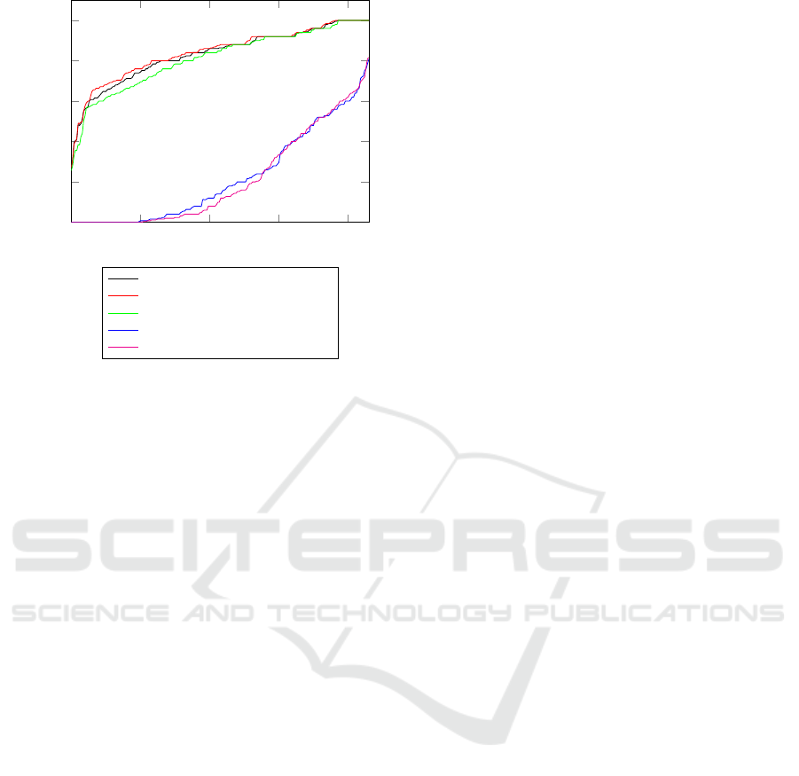
In order to get an overview of the suitability, 5

common dispersion metrics (cf. Fig. 2) were selected.

For each dataset, the mean precision was calculated

and then sorted in ascending order. It can be seen that

the variance, standard deviation, and median absolute

deviation perform signiﬁcantly better than the quartile

coefﬁcient of dispersion and coefﬁcient of variation.

As a consequence of this observation, it can be stated

that the variance and the standard deviation could pro-

vide the best results across all datasets. However,

since the standard deviation achieves slightly better

results for the datasets with lower achieved precision,

we decided to use the standard deviation as the basis

of the metric difference for further analysis.

4.2.2 Comparison of Datasets

In the second part of the evaluation, we took a closer

look at which datasets and dataset characteristics were

performing better or worse when identifying mean-

ingful features. This part of the evaluation was also

divided into large and small datasets according to

the above-mentioned characteristics. As described

in Sect. 2, Interpretable k-Means is the most simi-

lar algorithm to our approach. For this reason, In-

Increasing Explainability of Clustering Results for Domain Experts by Identifying Meaningful Features

369

100

150

200

0.2

0.4

0.6

0.8

Dataset

Mean Precision

Variance Difference

Standard Deviation Difference

Median Absolute Deviation Difference

Quartile coefﬁcient of dispersion Difference

Coefﬁcient of variation Difference

Figure 2: Evaluation of metrics on generated datasets.

terpretable k-Means was used to determine the mean

precision for each of the 216 datasets and used as a

baseline for evaluating our approach. The results for

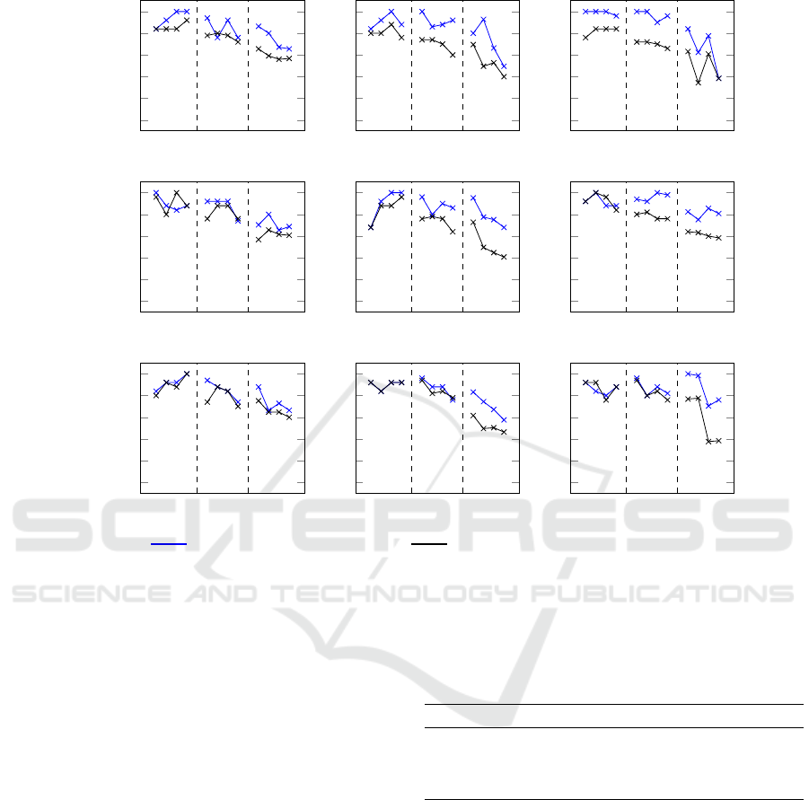
smaller datasets are shown in Fig. 3. This ﬁgure de-

scribes the mean precision achieved for each combi-

nation of the parameters. For instance, the sub-ﬁgure

at the top left shows the mean precision achieved for

5.000 instances and 10 features on the y-axis. In ad-

dition, the three different numbers of clusters c=5,

c=10, c=25 are depicted on the x-axis, and for each

of these combinations, the four possible noise ratios

from left (0) to right (0.99) are plotted. The results of

the baseline achieved with Interpretable k-Means are

depicted in black, while the results of our approach

are depicted in blue.

It is evident that in the vast majority of datasets

very good results could be achieved by our approach.

Only in a very limited number of parameter combina-

tions, the baseline was not met. Hence, the average

mean precision achieved by our approach across all

datasets is 0.85, i. e., at least 4 out of 5 meaningful

features were identiﬁed. The worst mean precision

achieved is around 0.4, which still leads to 2 meaning-

ful features that are found on average in each cluster.

The baseline, however, only achieves a mean preci-

sion of 0.74 on average. This means that on average

one meaningful feature less was identiﬁed. In addi-

tion, it was not possible to ﬁnd at least two meaning-

ful features in all of the examined datasets.

To demonstrate the performance of the approaches

from a user perspective, we also evaluated to what

extent a given minimum number of meaningful fea-

tures can be found with these approaches. If at least

4 meaningful features are to be identiﬁed, this re-

quirement is matched or exceeded in 81 of the 108

datasets by our approach, which is equivalent to a suc-

cess rate of 75 percent. For Interpretable k-Means,

this goal was only achievable in around 41 percent

of the datasets (45 datasets). If the rather implausi-

bly high noise of 66% or 99% additional instances

is not taken into account, the success rate of our ap-

proach increases to over 85 percent, i. e., 46 of 54

datasets with at least 4 out of 5 meaningful features,

for Interpretable k-Means the success rate in this con-

dition remains with 46 percent around the same level

(25 datasets).

Nevertheless, we expect that even less than 4

meaningful features support a domain expert in the

analysis tremendously. For instance, if a domain ex-

pert would be satisﬁed with a minimum of 3 mean-

ingful features, the success rate of our approach in-

creases to over 97 percent (105 out of 108 datasets).

If the excessive noise ratios are neglected, the success

rate even climbs to 100 percent. For Interpretable k-

Means, the requirement could be reached in signiﬁ-

cantly fewer datasets (48 of 108 datasets, 44 percent).

Here, when noise ratios are neglected the success rate

is still only at 88 percent (48 datasets).

Furthermore, it is apparent that as the noise ratio

increases, the results tend to get worse. Exceptions to

this pattern are the datasets with only a few features

and a small number of clusters. For these parameters,

adding random instances surprisingly leads to slightly

better results. However, it is not possible to draw a

clear correlation between individual parameters and

their inﬂuence on the achieved precision.

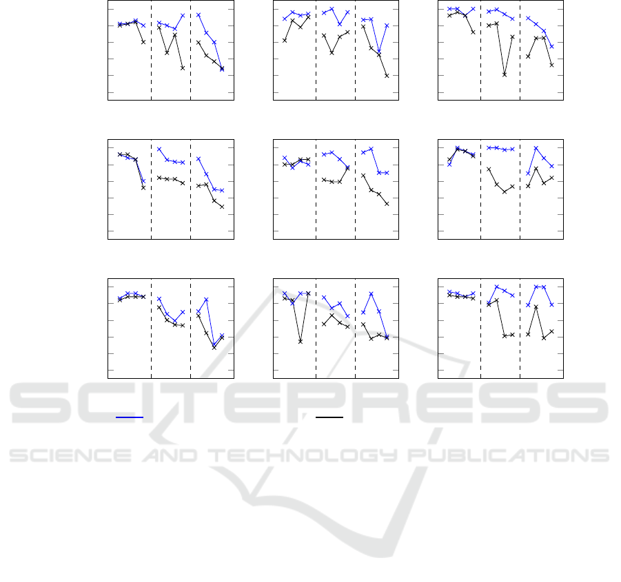
A similar general pattern is obtained when looking

at the results for the large datasets (cf. Fig. 4). Once

again, in the vast majority of the evaluated datasets

very good results could be achieved. In contrast to

the smaller datasets, the impact of the randomly gen-

erated additional noise is as expected. Although there

are occasional exceptions, noise generally causes a

decrease of precision in the results across all param-

eter combinations. In particular for large noise ra-

tios the precision drops signiﬁcantly in some cases

(e. g., f=25, n=100.000, c=50). Furthermore, it can

be seen that this effect weakens when considering a

larger number of features.

The average mean precision for the large datasets

achieved by our approach is approximately 0.83, with

0.27 in the worst case, i. e., we still identify more

than one meaningful feature in the worst case. In-

terpretable k-Means, in contrast, was able to achieve

a mean precision of 0.64 and 0.19 in the worst case,

i. e., there was again at least one dataset in which no

meaningful feature could be found.

ICEIS 2022 - 24th International Conference on Enterprise Information Systems

370

c=5 c=10 c=25

0.2

0.4

0.6

0.8

n = 5000

f = 10

c=5 c=10 c=25

0.2

0.4

0.6

0.8

f = 20

c=5 c=10 c=25

0.2

0.4

0.6

0.8

f = 40

c=5 c=10 c=25

0.2

0.4

0.6

0.8

n = 10000

c=5 c=10 c=25

0.2

0.4

0.6

0.8

c=5 c=10 c=25

0.2

0.4

0.6

0.8

c=5 c=10 c=25

0.2

0.4

0.6

0.8

n = 50000

c=5 c=10 c=25

0.2

0.4

0.6

0.8

c=5 c=10 c=25

0.2

0.4

0.6

0.8

Mean Precision of our approach Mean Precision of Interpretable k-Means

Figure 3: Overview of the mean precision achieved on smaller datasets. For each combination of instances n, features f and

clusters c the mean precision achieved with different noise ratios r (0, 0.33, 0.66, 0.99 from left to right) is shown.

In a head-to-head comparison, this implies that

our approach achieves the higher mean precision in 93

out of 108 datasets, i. e., in 86 percent of the datasets.

Looking at the results from a domain expert’s

perspective, our approach ﬁnds at least 4 meaning-

ful features in 72 percent of the datasets (78 out of

108), while Interpretable k-Means achieves this in

only 30 percent (33 out of 108 datasets). Without the

two greatest noise ratios, the success rate increases

to more than 83 percent (45 out of 54 datasets) for

our approach and again is limited for Interpretable k-

Means (37 percent, 20 out of 54 datasets). In the sce-

nario where the lower baseline of at least 3 meaning-

ful features is required, there is again a signiﬁcant in-

crease in the success rate using our approach. Across

all datasets, a success rate of more than 91 percent (99

out of 108 datasets) is achieved. Without the larger

noise ratios, the success rate is once again as for the

smaller datasets at 100 percent. These results were

not achievable with Interpretable k-Means. Across all

datasets, at least 3 meaningful features were found in

just 56 percent of the datasets (61 out of 108). Ex-

cluding the high noise ratios, this requirement was

achieved in 68 percent (37 out of 54 datasets). Ta-

ble 2 summarizes these results in comparison.

Table 2: Overview of the results achieved.

Mean 3 out of 5 4 out of 5

Interpretable k-Means (small) 0.74 44% (48/108) 41% (45/108)

Our approach (small) 0.85 97% (105/108) 75% (81/108)

Interpretable k-Means (large) 0.64 56% (61/108) 30% (33/108)

Our approach (large) 0.83 91% (99/108) 72% (78/108)

4.3 Discussion

In the ﬁrst part of our evaluation, a comparison of var-

ious dispersion metrics shows that the standard devi-

ation performs best. Here, the difference to the vari-

ance in the datasets with lower achieved mean pre-

cision is slightly surprising. A possible explanation

for this is that the variance is squared the standard

deviation value and thus deviations in the data are

taken into account more strongly. Thus, it is pos-

sible for outliers to be weighted strong enough that

they inﬂuence a meaningful feature to become a non-

meaningful feature or vice versa. Nevertheless, the

Increasing Explainability of Clustering Results for Domain Experts by Identifying Meaningful Features

371

c=10 c=25 c=50

0.2

0.4

0.6

0.8

n = 100000

f = 25

c=10 c=25 c=50

0.2

0.4

0.6

0.8

f = 50

c=10 c=25 c=50

0.2

0.4

0.6

0.8

f = 100

c=10 c=25 c=50

0.2

0.4

0.6

0.8

n = 500000

c=10 c=25 c=50

0.2

0.4

0.6

0.8

c=10 c=25 c=50

0.2

0.4

0.6

0.8

c=10 c=25 c=50

0.2

0.4

0.6

0.8

n = 1000000

c=10 c=25 c=50

0.2

0.4

0.6

0.8

c=10 c=25 c=50

0.2

0.4

0.6

0.8

Mean Precision of our approach Mean Precision of Interpretable k-Means

Figure 4: Overview of the mean precision achieved on large datasets. For each combination of instances n, features f and

clusters c the mean precision achieved with different noise ratios r (0, 0.33, 0.66, 0.99 from left to right) is shown.

ﬁrst part of the evaluation shows that the standard de-

viation is a well-suited metric due to similar values

at datasets with higher mean precision and better val-

ues at datasets with lower mean precision. Another

advantage is that the computation of the standard de-

viation is performed in linear time and oftentimes al-

ready computed anyway during the clustering algo-

rithm. Thus, there is at most a small overhead for our

approach to explain clustering results.

In the second part of the evaluation, the positive

effect of additional noise for smaller datasets is appar-

ent. The reason for this is unclear, but most likely it

is due to the fact that the equal distribution of the ad-

ditional instances makes the differences in the clean

data more obvious. Thus, for our chosen parameters,

there appear to be datasets in which there are too few

instances per cluster for the differences in a feature’s

value distribution to become apparent. This theory is

also supported by the fact that the effect actually only

occurs in the smaller datasets and is reversed in larger

datasets. In particular, with respect to the fact that our

approach is supposed to improve the interpretation by

a domain expert, this effect is not a real concern, since

the expert could be informed if there are too few in-

stances available in clusters. The achievable results

of our approach in both, smaller and larger datasets,

are quite good. We expect that any meaningful fea-

ture identiﬁed will already have a very positive effect

on the analysis and interpretation by a domain expert.

In the vast majority of 73 percent, even 4 out of 5

meaningful features are reliably identiﬁed. In order

to identify possible correlations, very large noise ra-

tios were also used for the evaluation, which are likely

to be encountered rather rarely in real-world data. Ac-

cordingly, success rates of 83 percent (90 out of 108

datasets with 4 out of 5 meaningful features) result

in the more realistic observations. For the mean pre-

cision of 3 meaningful features, which we consider

to be still very good, a success rate of 100 percent is

achieved. In particular, it should be mentioned that

there was not a single dataset in which the achieved

mean precision did not correspond to at least one

identiﬁed meaningful feature in each cluster. Given

this kind of noise, this speaks for very high robust-

ness, in particular, because very different scenarios

were tested in all possible permutations.

ICEIS 2022 - 24th International Conference on Enterprise Information Systems

372

In summary, the detailed results show that the

only comparable approach Interpretable k-Means was

outperformed by our approach in 93 percent of the

datasets. Moreover, Interpretable k-Means is con-

strained to k-Means, whereas our presented approach

works with any clustering result, regardless of the

conducted algorithm.

5 SUMMARY

In this paper, we introduced a new approach to in-

crease explainability for clustering algorithms. In the

ﬁrst step, we identify features that are most meaning-

ful for the interpretation of the clustering result based

on the analysis goals. Then, we determine a suitable

quantity of these meaningful features, which are still

comprehensible by domain experts. We apply statisti-

cal parameters to detail these features even more and

to decrease the interpretation complexity for domain

experts. Finally, we visualize the results by showing

the clusters and their corresponding meaningful fea-

tures to the domain experts, as well as by giving in-

sights in the concrete data characteristics, e. g., value

ranges, in the clusters. To assess the suitability of this

new approach, we conducted a comprehensive evalu-

ation based on 216 datasets. We show, that our new

approach is able to outperform existing solutions re-

garding the achieved precision in 93 percent of the

assessed datasets. Moreover, our new approach is ag-

nostic to the clustering algorithm used.

ACKNOWLEDGEMENTS

This research was performed in the project ’IMPORT’

as part of the Software Campus program, which is

funded by the German Federal Ministry of Education

and Research (BMBF) under Grant No.: 01IS17051.

REFERENCES

Alghofaili, Y. (2021). Interpretable K-means: Clusters fea-

ture importances. [Online: towardsdatascience.com].

Altmann, A. et al. (2010). Permutation importance: a cor-

rected feature importance measure. Bioinformatics,

26(10):1340–1347.

Behringer, M. et al. (2017). A Human-Centered Approach

for Interactive Data Processing and Analytics. In

ICEIS 2017, Revised Selected Papers. Springer.

Breiman, L. (2001). Random forests. Machine Learning,

45(1):5–32.

Cali

nski, T. and Harabasz, J. (1974). A Dendrite Method

For Cluster Analysis. Comm. in Statistics, 3(1):1–27.

Dasgupta, S. et al. (2020). Explainable k-means and k-

medians clustering. In Proc. of the ICML’20.

Davies, D. L. and Bouldin, D. W. (1979). A Cluster Separa-

tion Measure. IEEE Trans. Pattern Anal. Mach. Intell.

Dunteman, G. H. (1989). Principal components analysis.

Endert, A. et al. (2014). The human is the loop: new direc-

tions for visual analytics. J. Intell. Inf. Syst., 43(3).

Ester, M. et al. (1996). A Density-Based Algorithm for

Discovering Clusters in Large Spatial Databases with

Noise. In Proc. of the SIGKDD’96.

Fayyad, U. M. et al. (1996). From Data Mining to Knowl-

edge Discovery in Databases. AI Magazine, 17(3).

Fisher, R. (1988). IRIS Dataset. UCI ML Repository.

Frank, E. et al. (2016). The WEKA Workbench. Online Ap-

pendix for ”Data Mining: Practical Machine Learn-

ing Tools and Techniques”.

Hinton, G. and Roweis, S. T. (2002). Stochastic neighbor

embedding. In Adv. Neural Inf. Process. Syst.

Imhoff, C. and White, C. (2011). Self-Service Business In-

telligence. Best Practices Report, TDWI Research.

Jain, A. K. (2010). Data clustering: 50 years beyond K-

means. Pattern recognition letters, 31(8):651–666.

Keim, D. A. et al. (2008). Visual Analytics: Deﬁnition, Pro-

cess, and Challenges. In Information Visualization.

Kumar, V. and Minz, S. (2014). Feature selection: a litera-

ture review. SmartCR, 4(3):211–229.

Kursa, M. B. and Rudnicki, W. R. (2010). Feature selection

with the boruta package. J. Stat. Softw., 36(11):1–13.

Liu, Y. et al. (2013). Understanding and enhancement of

internal clustering validation measures. IEEE Trans.

on Cybernetics, 43(3):982–994.

Loyola-Gonz

alez, O. et al. (2020). An explainable artiﬁcial

intelligence model for clustering numerical databases.

IEEE Access, 8.

MacQueen, J. (1967). Some methods for classiﬁcation and

analysis of multivariate observations. In Proc. of the

Berkeley Symp. on Math. Stat. and Prob.

Maimon, O. and Rokach, L. (2010). Introduction to Knowl-

edge Discovery and Data Mining. In Data Mining and

Knowledge Discovery Handbook.

Miller, G. A. (1956). The magical number seven, plus or

minus two: Some limits on our capacity for processing

information. The Psychological Review, 63(2):81–97.

Rousseeuw, P. J. (1987). Silhouettes: A graphical aid to

the interpretation and validation of cluster analysis. J.

Comput. Appl. Math., 20(C):53–65.

Solorio-Fern

andez, S. et al. (2020). A review of unsuper-

vised feature selection methods. Artiﬁcial Intelligence

Review, 53(2):907–948.

Thorndike, R. L. (1953). Who belongs in the family? Psy-

chometrika, 18(4):267–276.

Wu, X. et al. (2008). Top 10 algorithms in data mining.

Knowledge and information systems, 14(1).

Increasing Explainability of Clustering Results for Domain Experts by Identifying Meaningful Features

373