A Performance Benchmark of Formulated Methods for

Forecast or Reconstruct Trajectories Associated to the

Process Control in Industry 4.0

Davi Neves

1 a

and Ricardo Augusto Rabelo Oliveira

2 b

Department of Production Engineering, University Federal of Ouro Preto, Ouro Preto, Brazil

Department of Computing Science, University Federal of Ouro Preto, Ouro Preto, Brazil

Keywords:

Dynamic Systems, Koopman Operator, Reinforcement Learning, Neural Networks, Topological Measures.

Abstract:

Manufacturing processes are generally modeled through dynamic systems, whose solutions establish a tool for

control theory, essential in the elaboration of industrial automation, a pillar of the fourth revolution. Under-

standing and mastering these technological procedures correspond to the ability to determine and analyze the

solutions of a system of differential equations, in order to deploy smart devices in a production line, such as the

robotic arm, because this trajectories can be always associated with the running of any equipment. Currently

there are many formulated methods to determine (or forecast) these curves, through numerical or stochastic

tools, the focus in this work are those capable of reconstructing a state space, such as the Koopman’s oper-

ator, convolutional neural network and reinforcement learning technique. Therefore, based on the solutions

provided by these methods, a benchmark will assembled to compare them, using topological measures such

as Shannon entropy, Lyapunov exponent and Hurst coefﬁcient, thus deﬁning the effectiveness of each one.

1 INTRODUCTION

The automation of manufacturing processes dates

back to the ﬁrst industrial revolution (Clark, 2014),

when thermal machines mechanized tasks once per-

formed by hands, expediting and improving industrial

production; now, facing the fourth revolution sup-

ported by electronic devices, an efﬁciency growing

is elucited and consequently to emerge greats chal-

lenges for scientists and engineers (Xu et al., 2018a;

Prisecaru, 2016; Xu et al., 2018b).

Primary challenge in the automaton process is the

ﬁt of its results, considering the input values in system

that represents this process; studies that approach this

topic are classiﬁed into the control theory, an applied

area of dynamical systems (Nise, 2020; Rodic, 2009),

which are formally represented by coupled differen-

tial equations (Haddad and VijaySekhar, 2011; Salle,

1976).

Normally, the control theory of automatized man-

ufacturing processes correspond to the solutions and

analysis of the differential equations that model them;

these systems are usually named like governing equa-

https://orcid.org/0000-0002-3144-0207

https://orcid.org/0000-0001-5167-1523

tions and their solutions are computed with numerical

methods (Stuart and Humphries, 1998; Beyn, 1991)

or block diagrams (Nise, 2020).

An ordinary differential equation express the be-

havior of a curve, this way the solution of coupled

equations correspond the union of distinct curves,

thus forming a n-dimensional surface known as man-

ifold. These structures are studied in topology, a the-

ory that provide tools to the understand of dynamic

systems (Akin, 2010; Materassi and Innocenti, 2010).

Curves (trajectories) referring to the solutions of

a dynamical system can be illustrated in state space,

rather than real space, because in this hidden symme-

tries are highlighted (Prince, 1982; Levi and Winter-

nitz, 1996). Koopman and von Neumann observed

this important detail and based on that they formu-

lated a theory (Koopman, 1931; v. Neumann, 1932a;

v. Neumann, 1932b) with enormous effectiveness and

usefulness for data-driven analysis (Williams et al.,

2015; Mezi

c, 2013; Proctor et al., 2018).

Using Koopman operator is possible to recon-

struct the trajectories in state space, which constitutes

a method to determine predictions regarding the sys-

tem’s behavior and hence a control tool for the cor-

responding process (Li and et al, 2017; Bruder et al.,

594

Neves, D. and Oliveira, R.

A Performance Benchmar k of Formulated Methods for Forecast or Reconstruct Trajectories Associated to the Process Control in Industry 4.0.

DOI: 10.5220/0011086800003179

In Proceedings of the 24th International Conference on Enterprise Information Systems (ICEIS 2022) - Volume 1, pages 594-601

ISBN: 978-989-758-569-2; ISSN: 2184-4992

2019).

Due to importance of this reconstruction process

other methods have been developed, among which it

is worth mentioning the Packard theory that use delay

coordinates (Packard and et al, 1980) and those that

use neural networks, with convolutional (Hauser and

et al, 2019; Teng and Zhang, 2019) or autoencoders

structures (Otto and Rowley, 2019; Almazova et al.,

2021; Champion and et al, 2019).

To complement the control theory approach ref-

erent to trajectories analysis, reinforcement learning

should also be included, because in this method the

most probable trajectory is determined by a Marko-

vian decision process. Although this methodology

(stochastic) is not in the same context (deterministic)

as the ones mentioned before, its leading objectives

are equivalents: compute the path most effective to

carry out a process (Sutton and Barto, 2018; Kael-

bling et al., 1996).

In order to elaborate an analysis that cover all

these methods, a robotic arm was selected like ob-

ject of study, due to your wide bibliographic reference

and the inherent complexity its mathematical model, a

double pendulum (chaotic behavior), thus warranting

the suitable requirements for build the benchmark.

We started with a theoretical review of dynamic

systems and their fasten relationship with process

control, followed by the Koopman operator approach,

in next section we present essential concepts about

models that use reinforcement learning and then we

complement the description of the methods to trajec-

tories rebuild with a decoder type neural network.

The theoretical overview will be concluded with

the presentation of the effectiveness measures, us-

ing topological methods such as Lyapunov exponent,

Hurst coefﬁcient and Shannon entropy (Akin, 2010);

we will also elucidate Pearson’s statistical coefﬁcient

(Montgomery et al., 2009), which makes it possible

to analyze the correlation between real and predicted

trajectories.

In results section we will present the simulation

environment, in which highlight the hardware and

softwares used, proceeding to the proposed analy-

ses, where we will evaluate the effectiveness of each

method mentioned, always establishing a relationship

with the robotic control.

2 DYNAMICAL SYSTEMS AND

CONTROL

Dynamical systems are essential in the control of in-

dustrial devices and processes, because their govern-

ing equations compose the theoretical formulation of

these events. Analysis can be performed through the

corresponding block diagram or by state space (Nise,

2020), for nonlinear equations the latter is the alter-

native most pertinent (Stuart and Humphries, 1998;

Beyn, 1991), since symmetries and topological mea-

sures are highlighted, which contribute signiﬁcantly

to the control of projects in industry 4.0 (Xu et al.,

2018a).

A trivial case study that provides the elucidation

of these controls is robotic arm, whose objective is

to reach a target and then move it; this process, or

device, can be modeled using equations that govern

the motion of a double pendulum, and despite being a

three-dimensional system, for simplicity without lose

the essence, can be modeled in two dimensions.

According to these considerations, the differential

equations must couple the angular variable (θ) and

their respective velocity (ω), resulting in complex ex-

pressions that can be presented in a concise way:

∂

∂t



θ,t,α



(1)

In (1) θ and ω are coupled into

θ vector, while

the equations system is represented by functional

named like ﬁeld, because it’s associated with the vec-

tor ﬁeld of the states space corresponding.

Time is illustrated by the dependent variable t and

the system parameters are represented by α; also, re-

garding (1), is worth noting that this system refers to

continuous states, for the discrete case a more ade-

quate formulation would be:

k+1

(2)

In the control theory θ

k+1

represents the output of

the system (posteriori signal) and θ

is called of input

(priori signal), while

F operator promote state evo-

lution (θ); to establish the control this operation must

be linearized, making outputs directly associated with

input signals, thus elucidating the scope of this theory.

For linear systems, the control methodology is al-

ready well established, so there are several tools, the-

oretical and practical, to adjust input signal until the

required output is obtained, within an acceptable mar-

gin of error, however, for nonlinear systems the inher-

ent complexities usually affect your control.

3 KOOPMAN OPERATOR

METHOD

Nonlinear systems are approached by control theory

from linearization methods, such as the Taylor se-

ries truncated, that has inspirited numerous and effec-

A Performance Benchmark of Formulated Methods for Forecast or Reconstruct Trajectories Associated to the Process Control in Industry

4.0

595

tive procedures, however, in this section, will be pre-

sented dimension reduction methods using coordinate

transformations, like the Packard’s work (Packard and

et al, 1980).

Packard’s work inspired others (Broomhead and

et al, 2020; Schmid, 2010), in which the dimen-

sion reduction, such as principal component analysis

(PCA), was combined with the fast Fourier transform

(FFT) to formulate what has been termed by dynamic

mode decomposition (DMD) (Proctor et al., 2018),

that therefore was associated with Koopman operator

(Koopman, 1931), method developed in 1931 for an-

alyze the time evolution of observables.



k+1



K.g





(3)

Fundamentally the Koopman operator (

K) works

in the space of observables, relatives to the system’s

states; considering that the dimension of this space is

inﬁnite, the linearization process will be feasible, thus

if the measure function was g





the evolution of the

observables will be given by equation (3).

The key point of this methodology is that even if

the operator

F, which represents the dynamical sys-

tem, was nonlinear, the Koopman operator will pro-

vide a linear way of time evolve states, thus enabling a

way to reconstruct the trajectories in respective states

space (control).

In its primordial practical formulation, the deter-

mination of the elements of this operator required an

adequate choice of basis functions for the proper rep-

resentation of the

K matrix, which was often infeasi-

ble, but currently the construction of these base func-

tions is referred to deep learning methods (Li and

et al, 2017), using neural networks to estimate their

eigenvectors and eigenvalues.

Addition to the use of deep learning, which ex-

panded the applicability of this method (Proctor et al.,

2018), in industry 4.0 context the control usually can

be data-driven (Li and et al, 2017), thus referring

to the DMD method, which enables the construction

of the Koopman operator using data series (Williams

et al., 2015):

K ≈

(4)

In (4)

is the matrix of posteriori states and

the Moore-Penrose pseudoinverse matrix of previous

states (

T ) (Mezi

c, 2013; Li and et al, 2017).

As the focus of this work is to evaluate method-

ologies for robot’s arm control, the Koopman opera-

tor will then be built using data from double pendu-

lum simulations, from ordinary differential equations

integration referring to this model.

4 REINFORCEMENT LEARNING

Among many machine learning techniques, control

theory can be meet on the reinforcement learning, in

which an agent interacts with the environment and as

result a learning is constituted, represented by a ta-

ble of rewards referred like Q-table (Sutton and Barto,

2018; Kaelbling et al., 1996).

Formally this learning process can be analyzed

from Bellman’s equation (Sutton and Barto, 2018),

referring to the current state-value ν(θ):

ν(θ) = max



R(θ,a) + γ.ν(θ

)



(5)

Agent’s action must maximize the sum between

the archived state-value ν(θ

) for all possibles next

states θ

and the current reward considering all pos-

sibles actions at state θ. Discount factor (γ) was in-

troduced to ν(θ) focus on immediate instead of future

rewards.

After this training, the most efﬁcient trajectory is

performed, or in other words the most probable path,

considering a policy π(θ/a) that deﬁnes the probabil-

ities of each action a in a respective state θ, then, set-

ting this methodology like this, your objective is ﬁnd

the optimum policy π which leads to the build of the

most probable trajectory for the robotic arm.

Although this description elucidates the similar-

ities between the methods discussed in this text, it

should be noted that in this case the essence of the

approach is stochastic, different from deterministic

character adopted by dynamical systems theory.

Currently, there have been improvements with the

use of neural networks, which replace the Q-table in

the agent’s learning process, that is, in the determina-

tion of the most probable trajectory. In this approach,

each agent state will be used as an input signal in

the neural network and the output will be the reward

referring to an action in this state (Kaelbling et al.,

1996).

In this work, trajectories for a robotic arm will

be constructed considering the previous knowledge of

the object’s position to build the Q-table, methods us-

ing the neural networks will also be evaluated, with

soft actor critic algorithm (SAC) (Sutton and Barto,

2018), that optimizes a stochastic off-policy, in order

to carry out the integration of this technique with oth-

ers, thus providing its improvement and expanding its

applicability.

ICEIS 2022 - 24th International Conference on Enterprise Information Systems

596

5 DECODER NEURAL

NETWORKS

Trajectories are essentially graphical representations

of a movement, due to this the most suitable neural

networks to deal with these are convolutional ones, as

will be explained in this section.

Without dodging of the work’s objective, the con-

volutional neural network (CNN) corresponds to a

structure in which an image will be initially polished

and ﬂattened, thus forming a ﬁrst-order tensor, ﬁtted

like an input signal of this neural network whose lo-

gistical output normally results in the classiﬁcation

this image (Teng and Zhang, 2019).

Although convolutional neural networks can be

used to analyze dynamical systems (Teng and Zhang,

2019; Otto and Rowley, 2019; Almazova et al., 2021),

the reconstruction of paths in the state space is more

consistent with the structure called like autoencoder

(ﬁg. 1-A), in which a neural network (encoder) com-

presses an image in a latent space to that then a second

network (decoder) make another image, correspond-

ing to the one used as input (Otto and Rowley, 2019;

Almazova et al., 2021).

(A)

(B)

Figure 1: Representation of neural networks structures, in

(A) an autoencoder is illustrated and in (B) the structure

used in this work.

As the purpose of this work is to analyze tech-

niques capable of reconstructing trajectories in the

state space and considering the high cost of autoen-

coders, a reduced structure was elaborated, consti-

tuted only by a network similar to the decoder (ﬁg.

1-B), using as latent space the initial conditions of the

problem in question, that is, the initial positions of the

object and robotic arm, producing as output an image

that illustrates a trajectory in state or real spaces.

Using several trajectories referring to different ini-

tial positions, for the target and robotic arm, a decoder

neural network was trained to construct (not recon-

struct) the trajectories relevant to the aforementioned

control. In the training, initial conditions were put

in the format of a 2x2 matrix, whose elements repre-

sented the positions of the arm and the object, then

this matrix was converted into the image of a trajec-

tory consistent with the pendulum solution.

6 TOPOLOGICAL MEASURES

Visual similarity (or difference) between two curves

can lead to hasty and wrong conclusions, with re-

gard to the evaluation of the reconstruction capacity

of a method, however topological analysis provides

tools to perform the appropriate analysis, with preci-

sion and efﬁciency.

Pearson’s correlation coefﬁcient may be the ﬁrst

tool used (Montgomery et al., 2009), because despite

its statistical formulation, its value indicates the co-

herence between two curves, that is, positive values

close to unity correspond to similar curves, on the

other hand, negative values close to unity indicate an

inverse behavior between two curves, ﬁnally, to the

other values no correspondence is veriﬁed.

ρ =

COV (θ

,θ

)

VAR(θ

).VAR(θ

)

(6)

The previous expression represents the calculation

of Pearson’s coefﬁcient, using the covariance between

two data series, the ﬁrst (θ

) correspond to original

trajectory and the second (θ

) to forecast (rebuild).

The denominator is deﬁned by the square root of the

variances referring to these trajectories.

Another important measure is Shannon entropy,

which deﬁnes the amount of information contained in

a data series, considering the occurrence of an event,

its basic formulation is as follows (Materassi and In-

nocenti, 2010):

S = log



i+1

i−1



(7)

In (7) P

i−1

is the priori probability of the event’s

occurrence and P

i+1

is the posteriori probability.

According to this formulation, is evident that this

value indicates the complexity of respective data se-

ries, as it quantiﬁes the information (bits) needed

to describe the occurrence of this event, however, it

should be noted that, in this work only the similarity

of these measures will be evaluated, as this qualitative

assessment is sufﬁcient for the proposed objectives.

Lastly, two other values will also be determined,

the larger Lyapunov exponent and the Hurst coefﬁ-

cient (Materassi and Innocenti, 2010), the ﬁrst being a

measure of data’s chaoticity and the second a measure

A Performance Benchmark of Formulated Methods for Forecast or Reconstruct Trajectories Associated to the Process Control in Industry

4.0

597

of its fractal dimension, which refers to the complex-

ity of this data series, however, in this work these val-

ues will be evaluated only qualitatively, that is, similar

values indicate similar trajectories.

7 RESULTS AND DISCUSSIONS

7.1 Simulation Environment

The results presented in this section were obtained

in a cluster assembled using the Docker engine soft-

ware, with hardware composed by Intel i7 processor

(3.8 GHz) and 16 GB of RAM, aided in graphics pro-

cessing by an Nvidia Jetson Nano card with 128 cuda

cores (1.4 GHz) and 4GB of RAM.

Codes developed in this work used a series of

python libraries, the standards Numpy, Scipy and

Matplotlib, for numerical and graphical functional-

ity. Koopman method was deployed using PyKoop-

man, neural networks were elaborated with PyTorch,

while reinforcement learning simulations it used Gym

and Stable-Baselines3. The topological measures was

computed with Nolds (Harris and et al, 2020; Virta-

nen and et al, 2020; Hunter, 2007; Paszke and et al,

2019; Sch

olzel, 2019).

(A) (B)

Figure 2: Simulation environment used, (A) the ﬁrst is an

elaboration with Numpy and Matplotlib. (B) The second is

called Reacher-v2, deployed in Gym using the Mujoco.

All trajectories that emulate the behavior of a

robotic arm were produced in two simulation envi-

ronments, the ﬁrst (ﬁg. 2-A) created by the authors

only with standard libraries, while the ﬁgure B was

elaborated into Gym library (with Mujoco (Todorov

et al., 2012)); in both there is a area that delimits the

target’s position.

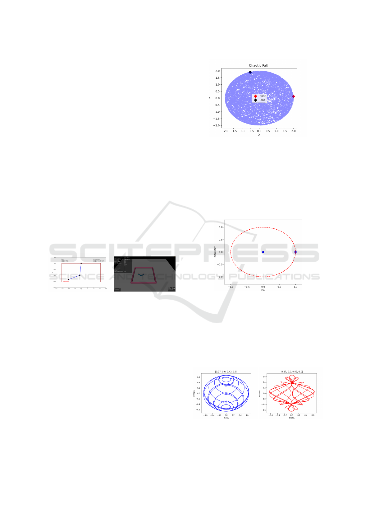
Movement of both emulators results in chaotic

paths that start at the initial position of the robotic arm

until it ﬁnds the target, whose position constitutes the

ﬁnal point, as is showed in ﬁgure 3.

7.2 Koopman Operator

Simulations referring to the Koopman method use nu-

merical solutions of the double pendulum like input,

Figure 3: Representation of a not optimized and chaotic

path generated by arm’s movement, simulated with double

pendulum equations.

computed with the Scipy module, from these trajecto-

ries and using PyKoopman module one can determine

the matrix corresponding to the operator.

Koopman eigenvalues are demonstrated in ﬁgure

4, which indicate that the eigenvectors neither grows

nor decay, that is, operator is stable, once it’s in your

adequate form to make forecast calculus.

Figure 4: Koopman operator eigenvalues, three are on the

unit circle and one is approximately zero.

The results illustrated in ﬁgure 5 represent trajec-

tories in the state spaces for the second joint angle

(θ

) and its respective velocity (ω

). In ﬁgure 5-A is

the result of the numerical integration, with mass and

length equal to one and using the initial conditions:

[0.27,0.0, 0.42, 0.0]. The second ﬁgure (5-B) is the

prediction using the Koopman operator.

(A) (B)

Figure 5: State space corresponding to the angle and its ve-

locity of the second joint. In (A) is the numerical solution

and in (B) the prediction respective.

ICEIS 2022 - 24th International Conference on Enterprise Information Systems

598

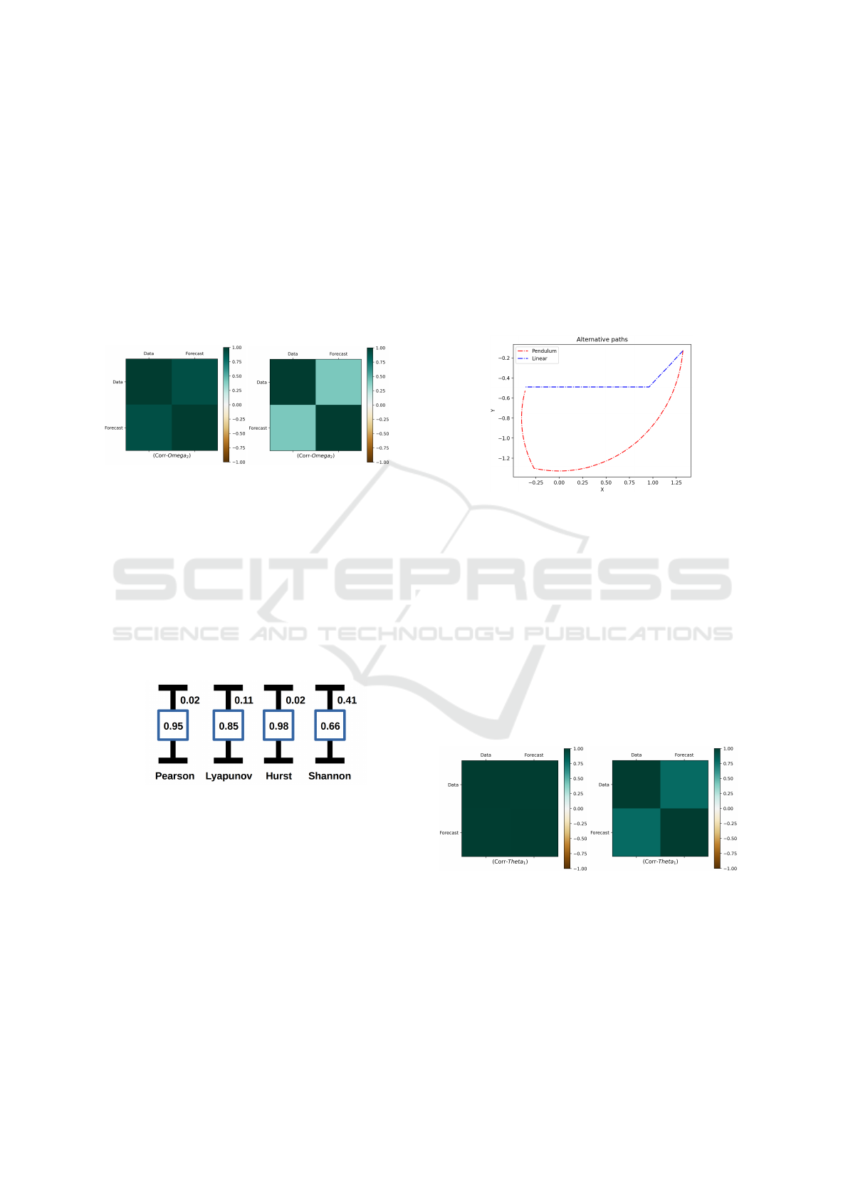
The Pearson correlation coefﬁcient for these two

state space trajectories is 0.94 (high), which indicates

a strong coherence between these curves, furthermore

is possible illustrate this result using a correlation ma-

trix (ﬁgure 6).

A particular result like the one illustrated in ﬁg-

ure 6-A can lead to wrong conclusions, then is impor-

tant to remember that a chaotic system is sensitive to

the initial conditions, as demonstrated by ﬁgure 6-B,

which is presented a correlation matrix for the system

that starts at [−0.32,0,0.64,0]. In this case the Pear-

son coefﬁcient is 0.36.

(A) (B)

Figure 6: (a) Correlation matrix for the trajectories illus-

trated in ﬁgure 5. (B) Correlation matrix for trajectories

with other initial conditions.

The curve with lowest Pearson coefﬁcient, pre-

sented a Hurst coefﬁcient of 0.93 for the actual data

and 0.94 for forecasts. The Shannon entropy for

the real data was 0.11 and for the predictions 0.15,

and ﬁnally the Lyapunov exponent in both cases was

slightly positive, conﬁrming the chaotic nature of this

system.

Figure 7: Normalized means and errors referring to topo-

logical and statistical measures.

An assemble to evaluate the data roughness was

elaborate from a sample with ﬁfty arbitrary initial

conditions, which was used to measure the efﬁciency

of the Koopman method, the statistical results are il-

lustrated in ﬁgure 7.

Analyzing the ﬁgure 7, was observe that Pearson

correlation coefﬁcient is positive and presents a error

(standard deviation) of 2%, while the Lyapunov expo-

nent presents a error of 11%, less stable. Hurst coef-

ﬁcient is very stable, with same error that the Pearson

coefﬁcient, lastly the Shannon entropy was the more

unstable, with a big error of 40%, which differs from

previous results.

7.3 Reinforcement Learning

To perform the reinforcement learning method, a dis-

crete state space was elaborated considering ﬁxed an-

gle step (dθ = 0.04) for each pendulum joints (θ

, θ

then a Q-table was determined, which induced to the

deploy of a space engine (DC motor) with constrains

movements, like a pendulum (ﬁg. 8), thus emulating

a deterministically programmed automaton system.

Figure 8: Trajectories for a robotic arm using reinforcement

learning (Linear/Blue) and the path like make by a DC mo-

tor (Pendulum/Red).

In each simulations was used the environment

called Reacher-v2, implemented in the Gym frame-

work (using Mujoco library), as this system is a con-

tinuous state space the SAC model was selected, so

that the SAC3 method, also deployed in this frame-

work, can be used too.

Neural network associated with reinforcement

method (SAC) was trained with 106 steps (workouts),

during this process were observed a convergence in

loss function from 20% of the training, then (1000)

tests were performed with 100% accurate results.

(A) (B)

Figure 9: Correlation matrix for the trajectories of rein-

forcement learng, with (A) high and (B) low coherence,

considering different initial conditions.

Similarly to the Koopman method, in this case the

Pearson coefﬁcient presented a small variation (1%),

thus demonstrating a strong coherence in the trajecto-

ries generated by this method; the others topological

A Performance Benchmark of Formulated Methods for Forecast or Reconstruct Trajectories Associated to the Process Control in Industry

4.0

599

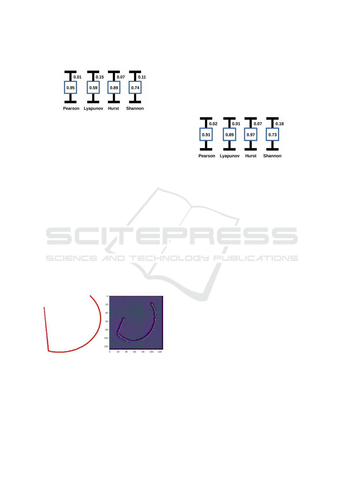
measures are shown in ﬁgure 10.

Figure 10: Normalized means and errors for topological and

statistical measures.

The Hurst coefﬁcient in this case varied more than

in Koopman method, between 0.85 to 0.92, i.e. 7%, as

illustrated in ﬁgure 10. Shannon entropy varied less

than before, around 11%, from 0.71 to 0.78. Lastly,

Lyapunov exponent again presented positives values,

but with the biggest error, around 15%. Overall, this

method performed better than the Koopman method.

7.4 Decoder Neural Network

The last method analyzed is a decoder neural network,

used to build trajectories from matrices that represent

the initial states, in this case the target and robot arm

positions:



target

arm



(8)

This initial matrix is ﬁrstly ﬂattened to one order

tensor, then passed through a neural network with 6

hide layers, the last one being an output with 3969

values. The output then goes through a process of

unpolishing and reshape for a 128x128 matrix, which

represents the trajectory predicted (ﬁg. 11-B).

(A) (B)

Figure 11: (a) Original pendulum trajectory, path from arm

(initial) to the target. (B) Results of the decoder neural net-

work after your training, with the same initial conditions.

In network training 5000 data were used, the su-

pervised learning was performed with one thousand

epochs and the loss function converged with approxi-

mately 600 steps. Next, the decoder then transformed

matrices like (8) in images as the ﬁgure 11-B, which

turn represent original pendulum trajectory, like illus-

trated in ﬁgure 11-A.

Fifty tests was performed using this neural net-

work, the results were further processed so that we

could determine the topological measurements; us-

ing the trajectories, predicted and original, was deter-

mined the topological measures for this method, thus

deﬁning its ability to reconstruct paths in state space.

Figure 12: Normalized means and standard deviations for

topological and statistical measures.

Analyzing the results (ﬁg. 12), can be observe

that the Pearson coefﬁcient is positive and with a very

small error (2%). The other values also presented

small errors, the Shannon entropy with a error of 18%

was the bigger. Lyapunov exponent and Hurst coefﬁ-

cient with 1% and 7% respectively, deviated less then

10%, which conﬁrm the effectiveness of this method.

8 CONCLUSIONS

According to the results presented in the previous ﬁg-

ures, it can be concluded that the topological measure-

ments showed that the methods evaluated are effec-

tive and despite the amplitude of the results the errors

were generally moderate.

Looking at ﬁgures 7, 10 and 12, it is worth not-

ing that the average Pearson coefﬁcient in all cases

is positive, indicating coherence between the original

and predicted curves. The errors of the other measure-

ments corroborate this statement, except for Shannon

entropy, which always exceeds 10%.

The chaoticity of this system justiﬁes the discrep-

ancies that occurred, it should still be noted that the

decoder neural network results were excellent, how-

ever this benchmark does not intend to point out the

best method.

Finally, as all methods were effective, it can be

concluded that all these are able to reconstruct a tra-

jectory for machine learning, thus stimulating their

association.

ICEIS 2022 - 24th International Conference on Enterprise Information Systems

600

REFERENCES

Akin, E. (2010). The general topology of dynamical sys-

tems. American Mathematical Society, Rhode Island,

USA.

Almazova, N., Barmparis, G. D., and Tsironis, G. P. (2021).

Analysis of chaotic dynamical systems with autoen-

coders. Chaos: An Interdisciplinary Journal of Non-

linear Science, 31.103109:1–10.

Beyn, W.-J. (1991). Numerical methods for dynamical sys-

tems. Advances in numerical analysis, 1:175–236.

Broomhead, D. S. and et al (2020). Singular system analysis

with application to dynamical systems. Chaos, noise

and fractals, pages 15–27.

Bruder, D., Remy, C. D., and Vasudevan, R. (2019). Nonlin-

ear system identiﬁcation of soft robot dynamics using

koopman operator theory. 2019 International Confer-

ence on Robotics and Automation. IEEE, pages 6244–

6250.

Champion, K. and et al (2019). Data-driven discovery of co-

ordinates and governing equations. Proceedings of the

National Academy of Sciences, 116.45:22445–22451.

Clark, G. (2014). The industrial revolution. Handbook of

economic growth, 2:217–262.

Haddad, W. M. and VijaySekhar, C. (2011). Nonlinear

dynamical systems and control. Princeton university

press, New Jersei, USA.

Harris, C. R. and et al (2020). Array programming with

numpy. Nature, 585:357–362.

Hauser, M. and et al (2019). State-space representations of

deep neural networks. Neural computation, 31:538–

554.

Hunter, D. (2007). Matplotlib: A 2d graphics environment.

Computing in Science & Engineering, 9.3:90–95.

Kaelbling, L. P., Littman, M. L., and Moore, A. W. (1996).

Reinforcement learning: A survey. Journal of artiﬁ-

cial intelligence research, 4:237–285.

Koopman, B. O. (1931). Hamiltonian systems and transfor-

mations in hilbert space. Proceedings of the National

Academy of Sciences, 17.5:315–318.

Levi, D. and Winternitz, P. (1996). Symmetries of discrete

dynamical systems. Journal of Mathematical Physics,

37.11:5551–5576.

Li, Q. and et al (2017). Extended dynamic mode decom-

position with dictionary learning: A data-driven adap-

tive spectral decomposition of the koopman operator.

Chaos: An Interdisciplinary Journal of Nonlinear Sci-

ence, 27.103111:1–10.

Materassi, D. and Innocenti, G. (2010). Topological iden-

tiﬁcation in networks of dynamical systems. IEEE

Transactions on Automatic Control, 55.8:1860–1871.

Mezi

c, I. (2013). Analysis of ﬂuid ﬂows via spectral proper-

ties of the koopman operator. Annual Review of Fluid

Mechanics, 45:357–378.

Montgomery, D. C., Runger, G. C., and Hubele, N. F.

(2009). Engineering statistics. John Wiley & Sons,

USA.

Nise, N. S. (2020). Control systems engineering. John Wi-

ley & Sons, New York, USA.

Otto, S. E. and Rowley, C. W. (2019). Linearly recurrent

autoencoder networks for learning dynamics. SIAM

Journal on Applied Dynamical Systems, 18.1:558–

593.

Packard, N. H. and et al (1980). Geometry from a time

series. Physical review letters, 45.9:712–716.

Paszke, A. and et al (2019). Pytorch: An imperative style,

high-performance deep learning library. Advances in

Neural Information Processing Systems, pages 8024–

8035.

Prince, G. E. (1982). Lie symmetries of differential equa-

tions and dynamical systems. Bulletin of the Aus-

tralian Mathematical Society, 25.2:309–311.

Prisecaru, P. (2016). Challenges of the fourth industrial rev-

olution. Knowledge Horizons - Economics, 8.1:57–

62.

Proctor, J., Brunton, S. L., and Kutz, J. N. (2018). Gener-

alizing koopman theory to allow for inputs and con-

trol. SIAM Journal on Applied Dynamical Systems,

17.1:909–930.

Rodic, A. (2009). Automation and Control: Theory and

Practice. InTech, Rijeka, Croatia.

Salle, J. P. L. (1976). The stability of dynamical sys-

tems. Society for Industrial and Applied Mathematics,

Philadelphia, USA.

Sch

olzel, C. (2019). Nonlinear measures for dynamical sys-

tems, volume 1ed. Zenodo.

Schmid, P. J. (2010). Dynamic mode decomposition of nu-

merical and experimental data. Journal of ﬂuid me-

chanics, 656:5–28.

Stuart, A. and Humphries, A. R. (1998). Dynamical systems

and numerical analysis. Cambridge University Press,

Cambridge, UK.

Sutton, R. S. and Barto, A. G. (2018). Reinforcement learn-

ing. Elsevier, Mountain View, USA.

Teng, Q. and Zhang, L. (2019). Data driven nonlinear dy-

namical systems identiﬁcation using multi-step cldnn.

AIP Advances, 9.085311:1–8.

Todorov, E., Erez, T., and Tassa, Y. (2012). Mujoco:

A physics engine for model-based control. 2012

IEEE/RSJ International Conference on Intelligent

Robots and Systems, pages 5026–5033.

v. Neumann, J. (1932a). Zur operatorenmethode in

der klassischen mechanik. Annals of Mathematics,

33.3:587–642.

v. Neumann, J. (1932b). Zusatze zur arbeit ,,zur operatoren-

methode... Annals of Mathematics, 33.4:789–791.

Virtanen, P. and et al (2020). Scipy 1.0: Fundamental al-

gorithms for scientiﬁc computing in python. Nature

Methods, 17.3:261–272.

Williams, M. O., Kevrekidis, I. G., and Rowley, C. W.

(2015). A data–driven approximation of the koop-

man operator: Extending dynamic mode decomposi-

tion. Journal of Nonlinear Science, 25.6:1307–1346.

Xu, L. D., Xu, E. L., and Li, L. (2018a). Industry 4.0: state

of the art and future trends. International Journal of

Production Research, 56.8:2941–2962.

Xu, M., David, J. M., and Kim, S. H. (2018b). The fourth

industrial revolution: Opportunities and challenges.

International journal of ﬁnancial research, 9.2:90–95.

A Performance Benchmark of Formulated Methods for Forecast or Reconstruct Trajectories Associated to the Process Control in Industry

4.0

601