Multivariate Interpolation at the Edge to Infer Faulty IoT Sensor Metrics

Marcos Paulo Konzen

1,4 a

, Patric Lincoln Ramires Izolan

1 b

, F

abio J

unior Griesang

1 c

Paulo Silas Severo De Souza

2 d

, Tiago Coelho Ferreto

2 e

, Arthur Francisco Lorenzon

3 f

Marcelo Caggiani Luizelli

3 g

, Julio Carlos Balzano De Mattos

4 h

, Cinara Ewerling Da Rosa

1 i

and F

abio Diniz Rossi

1 j

Federal Institute Farroupilha, Alegrete, Brazil

Pontiﬁcal Catholic University of Rio Grande do Sul, Porto Alegre, Brazil

Federal University of Pampa, Alegrete, Brazil

Federal University of Pelotas, Pelotas, Brazil

Keywords:

IoT, Modeling, Sensors, Simulation.

Abstract:

Virtual sensors are software entities that allow the estimation, through models, of critical variables in a given

environment. Metrics can be modeled computationally to estimate the values measured by a sensor without

installing it physically in the speciﬁed location. The monitoring and control of its variables by the edge are of

great importance, as they are directly related to increased productivity. This article presents the idea behind

virtual sensors, discusses some challenges and trends, presents such sensors’ modeling for estimating values,

and gives results based on a Smart Farming case study. The results show that the virtual sensors’ estimated

values are very close to reality, which shows that our method can be used with very high conﬁdence.

1 INTRODUCTION

Edge Computing (Mahmoudi et al., 2018) is a

paradigm that complements the Cloud Computing

model, aiming to process data on servers close to

users, that is, close to where data is generated and

consumed. In this way, data travels shorter distances,

which dramatically reduces latency to a few millisec-

onds. For this reason, Edge Computing is a cru-

cial factor in the consumption of data coming from

the Internet of Things (IoT). More and more sensors,

cameras, and systems will monitor the entire indus-

trial production process, evaluating and supervising

the equipment’s performance. All of this has as main

objectives: saving resources, decreasing the average

https://orcid.org/0000-0002-8765-970X

https://orcid.org/0000-0002-2391-7159

https://orcid.org/0000-0002-0136-3482

https://orcid.org/0000-0003-4945-3329

https://orcid.org/0000-0001-8485-529X

https://orcid.org/0000-0002-2412-3027

https://orcid.org/0000-0003-0537-3052

https://orcid.org/0000-0002-0619-9271

https://orcid.org/0000-0002-9077-5031

https://orcid.org/0000-0002-2450-1024

time spent on production, and raising the quality of

products. Sensors may measure position, tempera-

ture, pressure, and other physical or chemical param-

eters. A sensor is a technical component that converts

physical or chemical quantities in an electrical signal.

However, there are cases where the desired physical

amount cannot be measured directly through a physi-

cal sensor due to cost, energy, convenience, failure, or

other practical reasons, such as geography or space.

Based on these speciﬁc contexts, virtual sensors ap-

pear as a viable option.

This article introduces a new approach to estimate

values of a virtual position (so-called virtual sensor)

based on values collected from real sensors within

the same region. Our contributions can be summa-

rized as follows: (i) a multivariate interpolation model

for estimating values at positions addressed by vir-

tual sensors; (ii) a simulation for estimating the val-

ues assigned to virtual sensors, considering the phys-

ical sensors distributed in the environment; (iii) an al-

gorithmic implementation that allows using the pro-

posed mathematical model in real environments; and

(iv) evaluations of the proposed model against well-

known techniques in the literature, demonstrating the

advantages of the model presented in this article. Op-

280

Konzen, M., Izolan, P., Griesang, F., De Souza, P., Ferreto, T., Lorenzon, A., Luizelli, M., Balzano De Mattos, J., Ewerling Da Rosa, C. and Rossi, F.

Multivariate Interpolation at the Edge to Infer Faulty IoT Sensor Metrics.

DOI: 10.5220/0011084100003200

In Proceedings of the 12th International Conference on Cloud Computing and Services Science (CLOSER 2022), pages 280-287

ISBN: 978-989-758-570-8; ISSN: 2184-5042

timizing the farms’ production process is the main

reason for applying IoT to the production line. It al-

lows today’s equipment that makes up the farms’ in-

dustrial yard to be connected in a network. It means

that it makes all industrial machinery work automat-

ically using highly programmable intelligent sensors.

The main difference to the current scenario, which is

already packed with modern equipment, is that people

control these machines. With Smart Farms, the mar-

ket can expect in a few years that these machines will

be independent and interact with each other and with

the general farm system. It means that the equipment

will make decisions without human intervention.

2 VIRTUAL SENSORS

The virtual sensor is not a physical sensor but behaves

as such. Virtual sensors are software-driven models

that use available information from other measure-

ments and parameters to calculate an estimate of the

metric of interest, approximating the behavior of a

physical sensor. A virtual sensor can be created as

a function of other real physical sensors, and there

must be a correlation between the inputs and the vir-

tual sensor. A virtual sensor can simulate and replace

a real physical sensor through modeling that estimates

output values with the same reliability as a real sensor.

These sensors can act as a backup, where the use of a

physical sensor is made impossible by several factors

such as remote geographic location or sensor failure

(Liu et al., 2009).

Virtual sensor modeling can be based on empiri-

cal data, where historical data is used to derive a cor-

relation between outputs and inputs. It can be found

in analytics, which uses physical formulas for mod-

eling. The models proposed in the literature indicate

two ways virtual sensors provide values: analytical

and empirical models. In analytical models, the vir-

tual sensor calculates metrics based on physical laws.

In contrast, in empirical models experience is incor-

porated into the calculus (Liu et al., 2009). The deﬁ-

nition of the modeling technique depends on the sen-

sor design, application, and mathematical calculation

approach. Another goal of using virtual sensors is to

replace a physical sensor and its functions. In this

type of application, the main objective is to replace a

real sensor in case of failures or the impossibility of

installing a physical sensor on site. The related work

reveals that the application areas of virtual sensors are

quite different. We chose to classify applications into

large areas to facilitate visualization in this work.

• Industry: Virtual sensors are modeled to produce

new measurement data in order to improve pro-

duction processes (Shao et al., 2018). In (Tong

and Zewen, 2017) virtual sensors are created to

estimate measurements in places where it is not

possible to use a real sensor, for example, mea-

suring the performance of machines or measuring

chemical processes in oil extraction.

• Environment: Wang, Zhao, and Cui (Wang et al.,

2015) describe the use of virtual sensors to mon-

itor algal blooms. In (Asy’ari et al., 2019) virtual

sensors are used to measure solar radiation.

• Health: Erturk and Vollero (Erturk and Vollero,

2020) developed virtual sensors to improve surgi-

cal accuracy. In (Gupta and Mukherjee, 2016) vir-

tual sensors are used to monitor and predict hem-

orrhages in remote patients.

• Agriculture S

anchez-Molina (et al.) (S

anchez-

Molina et al., 2015) developed a virtual sensor

applied to monitoring the amount of water in the

biomass of the tomato crop. Moura (et al.) (Zhang

et al., 2020) uses virtualized sensors to provide

different measures of soil irrigation based on sta-

tistical data.

• Sensors-as-a-Service: This category appears as

a new trend in IoT. It creates virtual sensors to

make data from physical sensors available in the

cloud. In this way, different applications can use

data from these virtual sensors for their solutions

without the developer having access to the phys-

ical sensor (Fanti et al., 2018) (Ilyas et al., 2020)

(Flores et al., 2018).

Different virtual sensor modeling techniques are

presented in the literature. In this work, the modeling

techniques were divided into large areas to facilitate

work classiﬁcation as shown in Table 1.

Table 1: Virtual sensor modeling techniques.

Technique Article

Machine Learning Models

(Wang et al., 2015)

(Asy’ari et al., 2019)

(Yuan et al., 2020)

(Ilyas et al., 2020)

(Zhang et al., 2020)

Mathematical Models

(Cristaldi et al., 2020)

(Tong and Zewen, 2017)

(Fanti et al., 2018)

(Shao et al., 2018)

(Sutarya and Mahendra, 2015)

Generic Models

anchez-Molina et al., 2015)

(Gupta and Mukherjee, 2016)

(Flores et al., 2018)

(Erturk and Vollero, 2020)

Virtual sensor modeling applied in the industry

uses machine learning techniques or mathematical

models. Virtual sensors applied in Health and Agri-

culture mostly use modeling techniques based on

generic models. Finally, Sensor-as-a-Service is mod-

Multivariate Interpolation at the Edge to Infer Faulty IoT Sensor Metrics

281

eled using different types of modeling techniques.

Therefore, more and more virtual sensors are be-

ing implemented in various applications, and multiple

methods are used to model these sensors. However, it

is still a challenge to determine which modeling tech-

nique is the most suitable according to the type of ap-

plication, considering the types and amount of input

data of the models, the response time, and the compu-

tational resources needed for the modeling.

3 PROPOSED METHOD

The initial resource for a reﬁned development of the

numerical method is strongly associated with the de-

pendence on the location of the plotted mesh nodes

with a minimum number of elements. In this sense,

our proposal focus on discretizing the domain of a

simple geometric mesh in 2D through triangulation.

Therefore, we use concepts from the geometry of tri-

angles. For this, consider A = (x

, y

), B = (x

, y

)

and C = (x

, y

) the Cartesian coordinates of three

points of a plane where the area with the sign of a

triangle (S

ABC

) is given by:

ABC

det









. (1)

If the area of the triangle is null (S

ABC

= 0),

then the points A, B, and C are collinear (may be

coincident). This collinearity of the points is de-

ﬁned as a degenerated triangle and otherwise a non-

degenerated triangle. Additionally, if A, B and C are

arranged counterclockwise, we have S

ABC

= +∇ABC

and clockwise, S

ABC

= −∇ABC, where ∇ABC is the

conventional area of a triangle ∆ABC. This deﬁnition

introduces the decomposition property for the signed

area; that is, given a point P in the plane, there are

three other sub-triangles (∆PBC, ∆PCA, and ∆PAB).

Note that the sum of the areas of these sub-triangles

is equal to the area of ∆ABC. From there, it is possi-

ble to deﬁne whether the point P is located inside the

triangle ∆ABC. For this to occur, it is enough that all

areas of the sub-triangles are positive. Based on these

concepts, it is initially possible to identify the posi-

tion of the virtual sensor (P) concerning three physi-

cal sensors (A, B, and C). In the ﬁrst case, the point P

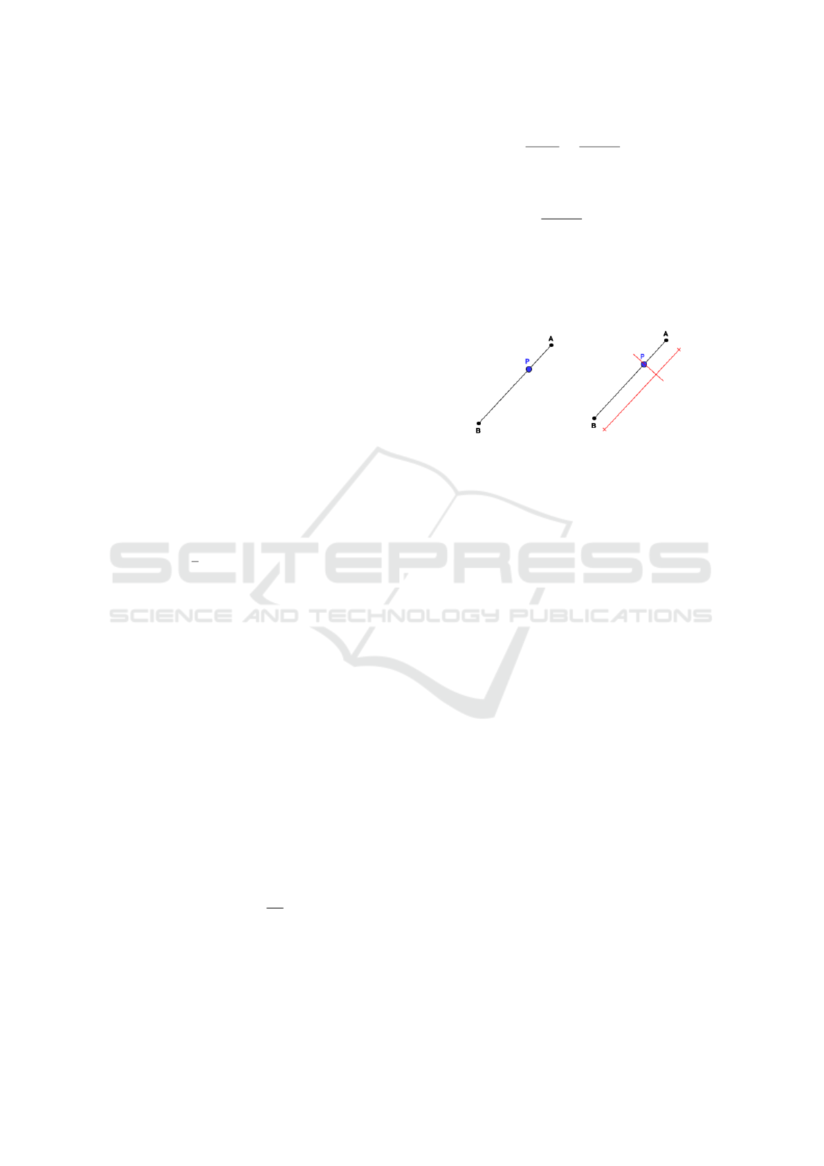
belongs to one of the segments of the ∆ABC; for ex-

ample, in Figure 1 where P ∈ AB, we have that ∆ABP

is deﬁned as a degenerated triangle. In this situation,

to estimate the position of the point P, the linear poly-

nomial interpolation method between the points A and

B (a ﬁrst-degree polynomial) will be used through the

following relation:

y − y

x − x

− y

− x

. (2)

Then

y = y

+ (y

− y

)

x − x

− x

at a point P = (x, y) (3)

which can be derived geometrically from Figure 1.

This function represents, by approximation, a sup-

posed function that would initially represent the im-

ages of a discontinuous interval contained in the do-

main.

(a) (b)

Figure 1: First case.

On the other hand, in the second case, the hypoth-

esis of a non-degenerated triangle ∆ABP is addressed;

it is assumed that P is not aligned to the points A and

B. Therefore, a new condition is assigned, requiring

this virtual sensor to triangulate among three physi-

cal sensors (A, B, and C). For this, the areas of the

sub-triangles must be all positive (Figure 2). If it is

identiﬁed that the point P is external to the triangle,

new vertices are assigned until the desired hypothe-

sis is found. In order to generate a mesh with good

formal patterns, the Delaunay method (Chew, 1989)

and the barycentric method (Pait, 2018) are initially

considered, which use the concept of dividing a no-

table point known as the barycenter. The barycen-

ter of the triangle is the noteworthy point of intersec-

tion of the three medians known as the center point

of weights. This method has an advantage in mesh

mapping as well as a good convergence acceleration

of the method. However, for the application of this

method, a reﬁnement of the mesh would be neces-

sary, with the use of successive points to obtain new

internal nodes in the mesh, deﬁned as a barycentric

subdivision. Note that the greater the number of ele-

ments in a mesh, the more costly and slower the com-

putational simulation. This situation is not interest-

ing for the feasibility of this study, which seeks to

interact in remote locations with low computational

resources. Given this fact, the option of this method

will be re-adapted to a technique that will reduce the

computational requirement and keep the data to a de-

sirable standard. However, the position of the vir-

tual sensor being restricted only to the barycenter of

CLOSER 2022 - 12th International Conference on Cloud Computing and Services Science

282

the physical sensors limits the problematization ap-

proach. In this sense, an alternative is to deﬁne the

point P from barycentric coordinates (u, v and w) in

relation to the triangle ∆ABC. It means that point P is

deﬁned through the weighted average of the vertices

of the triangle with weights u, v and w, that is,

P =

uA + vB + wC

u + v + w

= (u : v : w). (4)

Therefore, the proposed technique moves the

barycenter to the P point of interest, deﬁned by the

barycentric coordinate. Thus, it is possible to apply

multivariate interpolation (three linear interpolations)

based on the straight line from the angle that intersects

the opposite line.

Figure 2 demonstrates this process. In Figure 2

the point is deﬁned inside the triangle. In Figure 2 the

ﬁrst linear interpolation is performed. Figures 2 and 2

present the linear interpolation of the other two lines.

In the end, the three interpolated values are averaged

in order to estimate the value of the virtual sensor P.

4 EVALUATION AND

DISCUSSION

In this section, we evaluate the effectiveness of our

method in estimating the values of virtual sensors in

IoT environments. We start by describing our setup

(§4.2). We present the following experiments: (i)

we conduct a sensitivity analysis to ﬁnd the best set

of parameters to the compared algorithms (§4.3), and

(ii) we assess the performance of our proposal against

other algorithms (§4.4).

4.1 Case Study: Smart Farms

Population growth and technological advances have

led the agribusiness sector to invest in new meth-

ods, processes, and innovative equipment to produce

more and better. In practice, the Smart Farm con-

cept demonstrates these advances in the sector, where

information and communication technology has be-

come strong allies of rural producers. The purpose

of adopting this new farm concept is to improve efﬁ-

ciency and expand the sector’s productivity. The de-

mand for food has increased considerably, along with

the delivery speed (Memon et al., 2016). The Smart

Farm is based on the insertion of the countryside pro-

ducers and their activities in totally digital and in-

stantaneous information, enabling faster and more as-

sertive decision-making. For example, smart cameras

are already part of the farm’s reality. They have an

internal computer that can identify an image through

its format and colors and alert the farmer of possi-

ble risks to the plantation. When a threat appears, the

camera sends warning signals and messages via SMS,

email, and audible tones. With this, the producer can

avoid damage and take action quickly. Such threats

can be people wanting to steal supplies, equipments,

or even animals.

Another application is the use of drones in produc-

tion control and evaluation. The device, which can

be interconnected with a real-time image observation

system, has been used to detect pests, diseases, plant-

ing failures, and so on. From the top, the view of the

entire production is much broader and can be zoomed

in if necessary to observe some detail closely. By po-

sitioning the drone at the top, it is also possible to vi-

sualize the plant’s color, detect the presence of fungi,

and take photos to assist the agronomist in the analy-

sis. In addition, the drone also helps to monitor crop

development in real-time, making the analysis much

more effective than monitoring via car or motorcycle.

With the images captured, it is possible to carry out a

chronological analysis of the planting, helping devise

strategies for greater productivity, such as choosing

better soil collection points for analysis. Smart Farms

also may present built-in sensors at all stages of culti-

vation and in their equipment. In this way, when trav-

eling through the ﬁeld, they can collect different types

of data, such as light levels, soil conditions, irriga-

tion, air quality, and climate. The farmer can analyze

them and make preventive decisions based on these

data. Streamlining repetitive tasks also became possi-

ble through robots programmed through their sensors.

They entered data to walk across the entire ﬁeld and

work autonomously, weeding, watering, pruning, and

harvesting.

Sensors are often the smallest and most fragile

components of this intelligent environment. In most

cases, sensors are geographically distributed and ex-

posed to weather effects. It can lead to failures, and

consequently, impact productivity. Another factor

that this article addresses is those places that are dif-

ﬁcult to access and where it is not possible (or chal-

lenging) to place a sensor to carry out the measure-

ment, for example, very high treetops or at the bot-

tom of dams. It can delay or even derail important

alerts for the production environment. This article

aims to overcome the issues addressed above and pro-

poses modeling and estimating values through virtual

sensors that will be consumed by edge devices. The

proposed modeling is performed empirically, based

on values obtained from physical sensors around the

point of interest (virtual sensor). Virtual sensors are

not new within the ICT area (e.g., intelligent agents

Multivariate Interpolation at the Edge to Infer Faulty IoT Sensor Metrics

283

(a) (b) (c) (d)

Figure 2: Second case.

and monitoring software). Still, it has been emerging

as an option that ﬁts very well in IoT environments.

4.2 Experimental Setup

We compare our method with two well-known

distance-based data imputation techniques, k-Nearest

Neighbors (kNN) (Fix and Hodges, 1989), and In-

verse Distance Weighting (IDW) (Franke, 1982), and

a naive triangulation-based algorithm. Both kNN and

IDW estimate values based on the values of nearby

elements (in our context, physical sensors) with avail-

able data. While kNN estimates the values of virtual

sensors based on the arithmetic mean of the values

of their k nearest neighbors, IDW weights the known

observations of the k nearest neighbors based on their

distance to the virtual sensor so that closer neighbors

get more inﬂuence on the inference. The naive trian-

gulation algorithm iteratively creates a mesh of trian-

gles using the Delaunay algorithm and uses the ﬁrst

triangle it ﬁnds that surrounds the virtual sensor to es-

timate its value.

Our evaluation uses a real dataset with observa-

tions of 80 weather stations from the south region of

Brazil maintained by the National Institute of Mete-

orology (Inmet). Each weather station contains 8784

data points collected hourly during 2020 describing

temperature, atmospheric pressure, and relative air

humidity. According to INMET, this dataset is used

to drive strategic decisions in the country’s agriculture

sector. Table 2 presents statistical information about

the dataset. We intentionally omitted data from some

arbitrary weather stations in the dataset during the ex-

periments. After the tests, we compare estimated val-

ues from the evaluated techniques to the actual mea-

surements to assess the accuracy of inferences.

We evaluate the accuracy of compared techniques

based on two well-known error metrics: (i) Root

Mean Square Error (RMSE), which is given by

∑

i=1

( ˆy

−y

)

and measures the differences between

n predicted values ˆy and the expected values y based

on the square root of the average of squared er-

rors, and (ii) Mean Absolute Error (MAE), given by

∑

i=1

| ˆy

−y

, that measures the average of the abso-

lute errors. While both metrics help measure infer-

ences’ accuracy, a few large errors in a set of obser-

vations will increase the RMSE to a greater degree

than MAE, as it squares the differences before cal-

culating the average error. In our experiments, we

use MAE to account for the overall accuracy of the

techniques. At the same time, RMSE helps us iden-

tify the techniques’ ability to achieve steady results

while estimating the values of virtual sensors in dif-

ferent locations. We build a discrete-event simulator

that leverages object-oriented features of Python lan-

guage to mimic the behavior of weather stations from

the INMET dataset. We conducted the experiments

in a host machine with a quad-core Intel processor i7-

8650U@1.9GHz and 16GB of RAM running a Linux

Ubuntu 20.04.2 LTS (kernel 5.11.0-25-generic) and

Python 3.8.10. We assume that all of these algorithms

are present in the edge servers that collect the data

and can, in real-time, ﬁll the missing sensor data gap

with data from virtual sensors. Our simulator and the

dataset used during the tests are publicly available in

our GitHub repository

4.3 Sensitivity Analysis

Before comparing the algorithms, we evaluate how

the number of neighbors k affects the performance

of distance-based algorithms (kNN and IDW). To this

aim, we execute these algorithms with different val-

ues of k, assessing their RMSE and MAE in the three

evaluated scenarios. As shown in Figures 3 and 4, k =

8 leads to the best results for both algorithms when

estimating the values of virtual sensors regarding at-

mospheric pressure and temperature, which have less

dispersed data (see the standard deviation in Table 2).

In these scenarios, narrowing the number of neighbor

sensors used to perform inferences affects the accu-

racy of algorithms as sensor values are more or less

uniformly distributed based on their geographical po-

sition. On the other hand, k = 32 was the best pa-

rameter for estimating global solar radiation. Such a

scenario comprises more sparsed data, which favors

https://github.com/paulosevero/virtual-sensors-

triangulation

CLOSER 2022 - 12th International Conference on Cloud Computing and Services Science

284

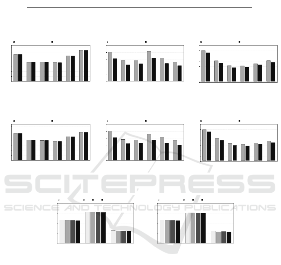
Table 2: Statistical information about the dataset.

Scenario Mean Standard Deviation Minimum Maximum

Temperature 13.9526 4.2081 -20.9 32.1

Atmospheric Pressure 960.8239 43.3078 811 1027.7

Global Solar Radiation 1467.0968 1111.4419 0 4806.6

27.69

19.54

19.82

19.30

26.21

31.91

27.69

19.54

19.82

19.30

26.21

31.91

1 2 4 8 16 32

Error

Number of Neighbors (k)

Root Mean Square Error (RMSE) Mean Absolute Error (MAE)

(a) Atmospheric Pressure

203

143

145

209

163

133

158

115

123

163

124

109

100

150

200

250

1 2 4 8 16 32

Error

Number of Neighbors (k)

Root Mean Square Error (RMSE) Mean Absolute Error (MAE)

(b) Global Solar Radiation

3.00

2.05

1.59

1.57

1.77

2.06

2.81

1.85

1.40

1.42

1.67

1.88

0.0

0.5

1.0

1.5

2.0

2.5

3.0

3.5

1 2 4 8 16 32

Error

Number of Neighbors (k)

Root Mean Square Error (RMSE) Mean Absolute Error (MAE)

Figure 3: Sensitivity analysis of k-Nearest Neighbors (kNN).

27.69

20.72

20.51

19.50

24.29

28.77

27.69

20.72

20.51

19.50

24.29

28.77

1 2 4 8 16 32

Error

Number of Neighbors (k)

Root Mean Square Error (RMSE) Mean Absolute Error (MAE)

(a) Atmospheric Pressure

203

145

141

181

158

138

158

117

121

141

120

106

100

150

200

250

1 2 4 8 16 32

Error

Number of Neighbors (k)

Root Mean Square Error (RMSE) Mean Absolute Error (MAE)

(b) Global Solar Radiation

3.00

2.18

1.70

1.62

1.74

1.92

2.81

1.98

1.52

1.47

1.63

1.77

0.00

0.50

1.00

1.50

2.00

2.50

3.00

3.50

1 2 4 8 16 32

Error

Number of Neighbors (k)

Root Mean Square Error (RMSE) Mean Absolute Error (MAE)

Figure 4: Sensitivity analysis of Inverse Distance Weighting (IDW).

21.26

128

1.89

19.30

133

1.57

19.50

138

1.62

18.24

122

1.56

100

1000

Atmospheric Pressure Global Solar Radiation Temperature

Root Mean Square Error

(RMSE)

Simple Triangulation kNN IDW Proposed Algorithm

(a) Root Mean Square Error (RMSE)

21.25

107

1.72

19.30

109

1.42

19.50

106

1.47

18.24

1.38

100

1000

Atmospheric Pressure Global Solar Radiation Temperature

Mean Absolute

Error

(MAE)

Simple Triangulation kNN IDW Proposed Algorithm

(b) Mean Absolute Error (MAE)

Figure 5: Accuracy results of the compared algorithms.

more neighbors during the inference of virtual sen-

sors.

4.4 Simulation Results

Looking at the results in Figure 5, we notice that the

error rates of all techniques grow more or less linearly

based on the degree of dispersion of data points of

the evaluated scenarios (atmospheric pressure, global

solar radiation, and temperature). Accordingly, all

strategies achieve higher accuracy when estimating

temperature and atmospheric pressure, as these sce-

narios have lower standard deviation than the global

solar radiation scenario. Among the compared meth-

ods, kNN and IDW were the most impacted by data

dispersion. They estimate the values of virtual sen-

sors based on the average values of k nearest sensors

with known data, which allows spread observations to

disturb their calculation. As such, kNN and IDW had

the worst results in terms of RMSE in global solar ra-

diation, as it presents the highest standard deviation

amongst the evaluated scenarios.

While kNN and IDW fall short on providing accu-

rate inferences about the global solar radiation of vir-

tual sensors, the triangulation-based methods manage

to get lower error rates by estimating the value of vir-

tual sensors based on reference points created with an

interpolation that is located closer to the virtual sen-

Multivariate Interpolation at the Edge to Infer Faulty IoT Sensor Metrics

285

sor than the physical sensors in the environment. The

main reason behind the superior results of the pro-

posed method against the Simple Triangulation relies

on which triangle is used to estimate the value of vir-

tual sensors. While Simple Triangulation picks the

ﬁrst triangle it ﬁnds surrounding the virtual sensor, the

proposed method goes further and looks for the trian-

gle comprised of physical sensors closer to the virtual

sensor. In that way, the proposed method manages

to get more accurate linear interpolations, resulting in

superior results (RMSE 4.87% lower than Simple Tri-

angulation).

When estimating the temperature of virtual sen-

sors, Simple Triangulation exhibited the worst re-

sults, ignoring the distance between the virtual sen-

sor and the points used in the triangulation. On the

other hand, the lower data dispersion in the dataset fa-

vored IDW and kNN that managed to get the third and

second-best results. Once again, the proposed method

achieved gains of 0.7% and 2.9% in terms of RMSE

and MAE compared to the second-best solution (in

this case, kNN) by inferring the value of virtual sen-

sors based on interpolated values of nearby reference

points within the triangles it generated.

4.5 Potential Impact on Smart Farms

The applicability of virtual sensors on smart farms al-

lows the analysis of data referring to a target without

direct contact with it through mathematical resources

based on real optical-electronic sensors. In addition,

virtual sensors will enable the creation and ﬁlling of

reliable data in maps of areas with no real sensors.

It is vitally essential for monitoring sparse areas and

over metrics measured by geographically remote de-

vices. Tools that use virtual sensors facilitate data

collection in the regions that are difﬁcult to access

and collaborate with the monitoring of dynamic pro-

cesses in nature. Several advantages make IoT-Edge

an important issue, especially in the current context

of society, as it can show geographic and historical

data relating to natural and social spaces. In addi-

tion, we currently discuss environmental preservation

as a global agenda in various educational and political

events around the globe and used in the monitoring

and analysis of natural resources. Among the most

relevant areas in which virtual sensors can positively

affect production.

One of the leading practices of virtual sensors is

associated within its use in Agriculture, as this tech-

nology has great potential, as it is possible to obtain

various information such as estimated planted area,

plant and crop health, pest detection in the planta-

tion, and observation of the production process, plant

counting, soil cover analysis, etc. The virtual sen-

sor can become one of the main tools of precision

agriculture because monitoring agricultural produc-

tion can provide productivity results never achieved

and reduce several operating costs. In addition, vir-

tual sensors can be used to analyze and monitor risk

areas, enabling the control of hurricanes, erosion,

and ﬂoods through satellite images and geoprocessing

techniques and the meteorological monitoring of the

earth and follow natural events. Through aerial im-

ages, it is also possible to assess the impacts of natural

disasters and allow strategies for prevention, combat,

and rescue. For example, drones with multispectral

cameras can identify hot spots in cave-in zones and

indicate survivors.

For forest areas, virtual sensors can be used to an-

alyze data regarding the distribution of forest areas,

advance deforestation activities, calculate volumes,

identify species, etc. Considering how relevant the

theme of environmental preservation has become in

recent years, especially in the world’s political en-

vironment, virtual sensors can become a fundamen-

tal tool for decision-making in the management and

management of natural resources, such as analyzing

and monitoring water resources, calculating and es-

timate physical and chemical parameters of soil and

water, determine the climatic characteristics of a re-

gion, identify critical points in anthropized areas, de-

termine the region’s relief, observe the behavior of

fauna in a region of interest, etc.

5 CONCLUSION AND FUTURE

WORK

Virtual sensors have internally implemented a model

with secondary input variables that can be measured

and output the variable of interest inferred. A virtual

sensor can infer values from positions where there

are no real sensors or where real sensors are inactive.

In this work, we proposed new modeling and imple-

mentation of virtual sensors based on the real sensor

values consumed by edge servers. The results of our

model were superior in terms of accuracy compared to

proposals in the literature based on IoT-Edge ecosys-

tems. To test our proposal, we used a well-know IoT

environment, a Smart Farm scenario.

Based on simulations using real-world traces, we

observe that our method can estimate the value of vir-

tual sensors with a high degree of accuracy, reducing

the RMSE and MAE by up to 5.5% and 5.8%, re-

spectively, compared to existing approaches. In fu-

ture work, we intend to incorporate a multivariate

technique that uses multiple correlated variables from

CLOSER 2022 - 12th International Conference on Cloud Computing and Services Science

286

nearby locations to estimate the value of virtual sen-

sors.

ACKNOWLEDGEMENT

This work was ﬁnanced in part by the Coordenac¸

de Aperfeic¸oamento de Pessoal de N

ıvel Superior -

Brasil (CAPES) – Finance Code 001. Also, this work

was partially supported by Conselho Nacional de

Desenvolvimento Cient

ıﬁco e Tecnol

ogico – CNPq

– 313111/2019-7. This work also received fund-

ing from S

ao Paulo Research Foundation (FAPESP)

– 2018/23092-1, 2020/05183-0, 2020/05115-4; and

Rio Grande do Sul Research Foundation (FAPERGS)

– 19/2551-0001266-7, 19/2551-0001224-1, 19/2551-

0001689-1, 21/2551-0000688-9.

REFERENCES

Asy’ari, M. K., Musyafa’, A., Noriyati, R. D., and Indri-

awati, K. (2019). Soft sensor design of solar irra-

diance using multiple linear regression. In 2019 In-

ternational Seminar on Intelligent Technology and Its

Applications (ISITIA), pages 56–60.

Chew, L. P. (1989). Constrained delaunay triangulations.

Algorithmica, 4(1-4):97–108.

Cristaldi, L., Ferrero, A., Macchi, M., Mehrafshan, A., and

Arpaia, P. (2020). Virtual sensors: a tool to improve

reliability. In 2020 IEEE International Workshop on

Metrology for Industry 4.0 IoT, pages 142–145.

Erturk, M. A. and Vollero, L. (2020). Gsp for virtual sen-

sors in ehealth applications. In 2020 IEEE 44th An-

nual Computers, Software, and Applications Confer-

ence (COMPSAC), pages 1683–1688.

Fanti, M. P., Mangini, A. M., Roccotelli, M., Nolich, M.,

and Ukovich, W. (2018). Modeling virtual sensors for

electric vehicles charge services. In 2018 IEEE Inter-

national Conference on Systems, Man, and Cybernet-

ics (SMC), pages 3853–3858.

Fix, E. and Hodges, J. L. (1989). Discriminatory analy-

sis. nonparametric discrimination: Consistency prop-

erties. International Statistical Review/Revue Interna-

tionale de Statistique, 57(3):238–247.

Flores, H., Hui, P., Tarkoma, S., Li, Y., Anagnostopoulos,

T., Kostakos, V., Luo, C., and Su, X. (2018). Sen-

sorclone: A framework for harnessing smart devices

with virtual sensors. In Proceedings of the 9th ACM

Multimedia Systems Conference, MMSys ’18, page

328–338, New York, NY, USA. Association for Com-

puting Machinery.

Franke, R. (1982). Scattered data interpolation: tests

of some methods. Mathematics of computation,

38(157):181–200.

Gupta, A. and Mukherjee, N. (2016). Rationale behind the

virtual sensors and their applications. In 2016 Interna-

tional Conference on Advances in Computing, Com-

munications and Informatics (ICACCI), pages 1608–

1614.

Ilyas, E. B., Fischer, M., Iggena, T., and T

onjes, R. (2020).

Virtual sensor creation to replace faulty sensors us-

ing automated machine learning techniques. In 2020

Global Internet of Things Summit (GIoTS), pages 1–6.

Liu, L., Kuo, S. M., and Zhou, M. (2009). Virtual sensing

techniques and their applications. In 2009 Interna-

tional Conference on Networking, Sensing and Con-

trol, pages 31–36.

Mahmoudi, C., Mourlin, F., and Battou, A. (2018). Formal

deﬁnition of edge computing: An emphasis on mo-

bile cloud and iot composition. In 2018 Third Inter-

national Conference on Fog and Mobile Edge Com-

puting (FMEC), pages 34–42.

Memon, M. H., Kumar, W., Memon, A., Chowdhry, B. S.,

Aamir, M., and Kumar, P. (2016). Internet of things

(iot) enabled smart animal farm. In 2016 3rd Inter-

national Conference on Computing for Sustainable

Global Development (INDIACom), pages 2067–2072.

Pait, F. M. (2018). The barycenter method for direct opti-

mization. arXiv preprint arXiv:1801.10533.

Shao, W., Chen, S., and Harris, C. J. (2018). Adaptive soft

sensor development for multi-output industrial pro-

cesses based on selective ensemble learning. IEEE

Access, 6:55628–55642.

anchez-Molina, J., Rodr

ıguez, F., Guzm

an, J., and

Ram

ırez-Arias, J. (2015). Water content virtual sen-

sor for tomatoes in coconut coir substrate for irriga-

tion control design. Agricultural Water Management,

151:114–125. New proposals in the automation and

remote control of water management in agriculture:

agromotic systems.

Sutarya, D. and Mahendra, A. (2015). Virtual sensor for

time series prediction of hydrogen safety parameter

in degussa sintering furnace. In 2015 2nd Interna-

tional Conference on Information Technology, Com-

puter, and Electrical Engineering (ICITACEE), pages

81–86.

Tong, W. and Zewen, D. (2017). Soft sensor modeling

method of dynamic liquid level based on improved ks

algorithm. In 2017 29th Chinese Control And Deci-

sion Conference (CCDC), pages 6510–6515.

Wang, Z., Zhao, Z., Li, D., and Cui, L. (2015). Data-

driven soft sensor modeling for algal blooms moni-

toring. IEEE Sensors Journal, 15(1):579–590.

Yuan, X., Zhou, J., Huang, B., Wang, Y., Yang, C., and

Gui, W. (2020). Hierarchical quality-relevant feature

representation for soft sensor modeling: A novel deep

learning strategy. IEEE Transactions on Industrial In-

formatics, 16(6):3721–3730.

Zhang, M.-Z., Wang, L.-M., and Xiong, S.-M. (2020). Us-

ing machine learning methods to provision virtual sen-

sors in sensor-cloud. Sensors, 20(7).

Multivariate Interpolation at the Edge to Infer Faulty IoT Sensor Metrics

287