Extracting Mass Transportation Networks from General Transit Feed

Speciﬁcation Datasets

Gergely Kocsis

and Imre Varga

Department of IT Systems and Networks,

University of Debrecen, Kassai str. 26, Debrecen, Hungary

Keywords:

GTFS, Public Transport, Networks.

Abstract:

In several smart-city applications the networks of the mass-transportation systems can be bases of investi-

gations. In this paper we show how one can extract a network of connected stops from the General Transit

Feed Speciﬁcation (GTFS) feed of a given service provider. We have also implemented this process as a tool

(gtfs2net) that is available for use at the GitHub page of the project. On of our most important ﬁnding is

that since providers do not follow the speciﬁcation in a coherent way regarding the use of parent stations the

problem of close stops has to be manually handled. In order to show how our tool works in practice we have

provided some extracted networks with their properties.

1 INTRODUCTION

Investigation of abstract networks of mass transporta-

tion providers is used frequently in smart city appli-

cations (Besenczi et al., 2021). Finding these net-

works however is not always trivial. There are sev-

eral maps online (even some that are free and open to

be used) that contain location of stops as well. From

these sources it is possible to get a network of stops

where the connection between them may be described

by some sort of physical relation (e.g. a connect-

ing road). In many cases however it is much reason-

able to name two stops connected if there is a direct

bus/tram/train trip between them.

One possible solution may be the use of the Gen-

eral Public Transit Feed Speciﬁcation (GTFS) de-

scribed timetables of transportation service providers.

The General Transit Feed Speciﬁcation is a current

format for public transportation schedules and the re-

lated geographic information (Harrelson, 2021). Be-

sides the opportunity of public transit agencies to pub-

lish their own transit data it lets software developers

to write applications that use this data to help users

in their daily lives. Numerous agencies provide their

public GTFS datasets, but they create them in differ-

ent manner (Wessel and Farber, 2019; Hansson et al.,

2019; Kujala et al., 2018a; Sienkiewicz and Hołyst,

https://orcid.org/0000-0003-0018-4201

https://orcid.org/0000-0003-3921-2521

2005; Braga et al., 2014). The native analysis of

these sources is already a widely studied topic by the

networks scientist comunity (Vuurstaek et al., 2020;

Fortin et al., 2016; Wong, 2013; von Ferber et al.,

2007; Gallotti and Barthelemy, 2015; Jiang, 2007;

ammer et al., 2006; Porta et al., 2006). However the

extraction of abstract networks from these sources is a

much less known ﬁeld. Moreover in most cases even

if the extracted networks are available the process is

not or only partially published (Kujala et al., 2018b).

In a simple GTFS based application a public trans-

port stop is just a geographical location with a few

meters in dimension. The feeds describe the connec-

tions of the stops as well. For a passenger however,

who travels probably some kilometers, a short walk

can be also included into the journey. This results in

connections between close stops, which are not con-

nected by the ofﬁcial datasets. As we found, it is

much harder to ﬁnd sources to build such networks

on this basis.

Below we will show how one can extract abstract

transportation networks from these feeds. In Section

2. we brieﬂy introduce the important parts of the spec-

iﬁcation. In Sections 3 and 4 we show the process

and the implementation aspects how to extract such

an abstract network from a provided feed. In Section

5 we show some basic properties of some extracted

networks to give an example how these networks can

later be used. Finally in Section 6 we conclude our

work and present our future plans.

Kocsis, G. and Varga, I.

Extracting Mass Transportation Networks from General Transit Feed Speciﬁcation Datasets.

DOI: 10.5220/0011080700003197

In Proceedings of the 7th International Conference on Complexity, Future Information Systems and Risk (COMPLEXIS 2022), pages 85-91

ISBN: 978-989-758-565-4; ISSN: 2184-5034

2 GENERAL TRANSIT FEED

SPECIFICATION

In the last 15 years the General Transit Feed Spec-

iﬁcation (GTFS) become the de-facto standard for

describing timetables of public transportation ser-

vices. The static component of the GTFS consists

of comma-separated values in simple text ﬁles con-

tained within a ZIP ﬁle. Each line of a ﬁle contains

a record of the given data table, covering various re-

quired and optional ﬁelds. There are mandatory and

optional ﬁles in the dataset. This section focuses on

just some of the ﬁles.

• stops.txt: It describes locations (e.g. stops, sta-

tions) related to the public transportation network

(PTN). Besides the ofﬁcial name of the place and

its precise latitude and longitude other informa-

tion can be stored in a record. One of these is the

parent station which can be used to deﬁne rela-

tionship among stops, platforms or boarding areas

of the premise.

• trips.txt: The trips are directional sequences

of stops connected by a transit vehicle during a

speciﬁc time period.

• routes.txt: A transit route is a directionless set

of trips concerning the same stops, so these trips

are displayed to riders as a single service.

• stop_times.txt: Times when a vehicle arrives

at and departs from stops for all the trips. These

records connect the trips, the stops and timing in-

formation.

The records of the ﬁles are interconnected by identi-

ﬁers. Stop time records contains stop id and trip id

ﬁelds in order to connect to the respective records.

The route id ﬁeld joins the routes and trips.

3 EXTRACTING ABSTRACT

TRANSPORTATION

NETWORKS FROM GTFS

FEEDS

Even though the original aim of GTFS is to provide a

standard for describing several aspects of public trans-

portation for network scientists one of the most prac-

tical use of it is that an abstract transportation network

can be extracted from the feed. However getting such

a network is not as trivial as one would think at the

ﬁrst sight mostly because of two problems: i.) Lo-

cal Transportation Providers sadly do not follow the

speciﬁcation fully in all cases or they follow it in dif-

ferent ways. ii.) It is not always exact what network

scientists would like to mean under a node or an edge

of the network.

To see the full picture let us see what is needed to

build a network in an ideal case. Our desired network

will have stops as its nodes and edges describing that

any time in the timetable there is a direct connection

between two stops. Thus to get the nodes we need

to process the stops.txt ﬁle of the GTFS feed. Be-

side several other ﬁelds, a record containing a stop has

the id of the stop (stop id) serving as the unique iden-

tiﬁer of it. In cases when we have only standalone

stops and no groups of stops are presented this ﬁeld is

enough to have a node. However in many cases some

of the stops are grouped because e.g. they are parts of

a bigger station. This relation is described by the lo-

cation type and the parent station ﬁelds of the record.

For an ordinary stop, the location type is 0. If it is

a part of a bigger station its parent station ﬁeld con-

tains a stop id referring to the parent stop. A parent

stop (parent station) has a location type of 1. Note

that the location type of a stop can also take values of

2, 3 and 4 but as practice shows these values are much

less commonly used.

Giving an answer to the ﬁrst above raised question

the nodes of our abstract network can usually be the

stops except in cases when a stop is contained by a

parent station. In this latter case the station itself can

be the node instead.

As mentioned above the edges of an abstract net-

work should be the connections between the stops.

unfortunately this information is not stored directly

in the datasets. The easiest way to get it is to pro-

cess the stop_times.txt ﬁle. In this ﬁle a stop of a

trip of a vehicle is described in each record. After the

ﬁelds describing the trip’s properties the stop id ﬁeld

here describes in which stop the vehicle stops. The

stop sequence tells what is the number of the stop in

the trip. It is easy to understand therefore if we have

read two records of the same trip with consecutive se-

quence numbers the stops mentioned in these records

can be treated as being neighbors in a way that there

is a directed edge from the stop with the smaller se-

quence number to the other.

The problem with the above described method of

ﬁnding edges is that it does not count with the pres-

ence of parent stations. This means that for example if

we have two stations with let us say three stops in both

that are connected by some trips directly, we will not

get a network with two nodes and two directed edges,

but we will get eight nodes some edges directly be-

tween the stops of the stations and no edges between

the stations themselves. Referring to the stops and

stations this way is however misleading in most of the

cases, so we suggest to use the parent stations of those

COMPLEXIS 2022 - 7th International Conference on Complexity, Future Information Systems and Risk

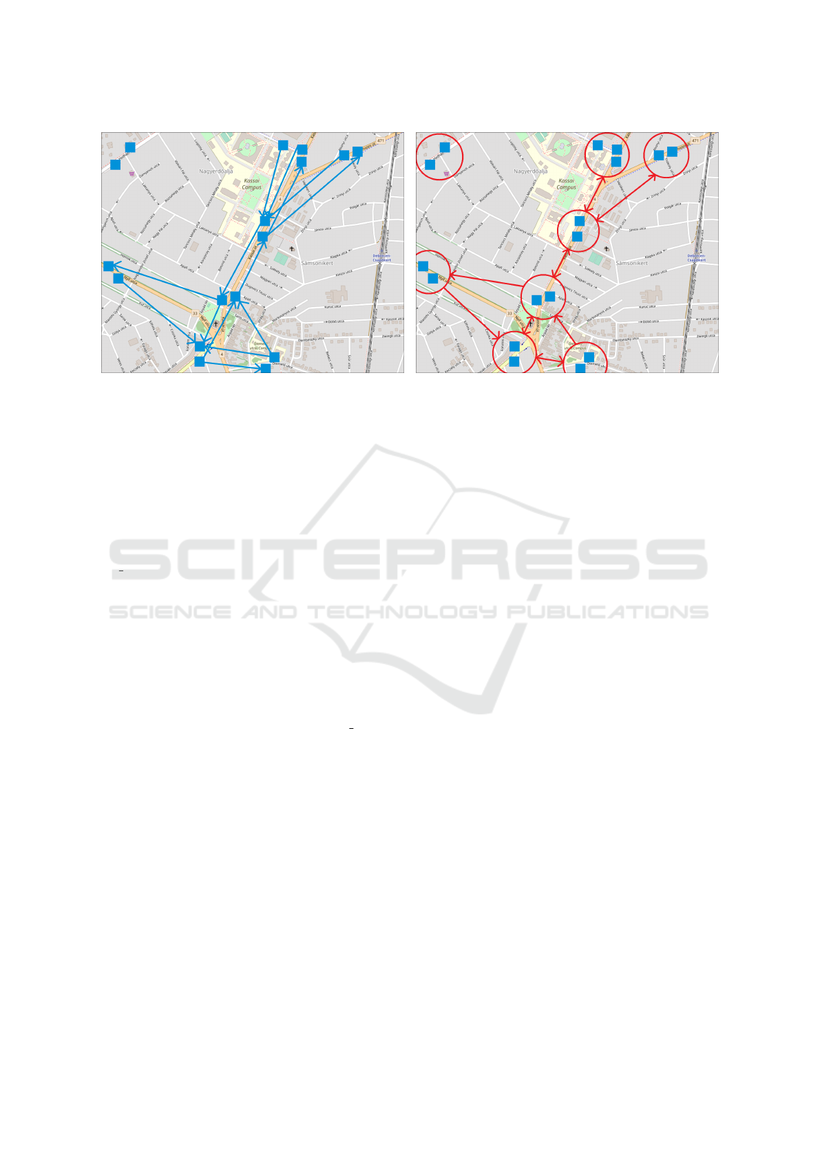
Figure 1: The effect of using virtual stations on the abstract topology of bus stations. left: Bus stations (blue squares) around

Debrecen University IT Campus and their connections (blue arrows). right: Stops merged by virtual stations (red circles) and

their connections (red arrows). (Picture source: OpenStreetMap.org).

stops that have one as the ends of these edges without

allowing the presence of multi-edges.

Extracting a network from a GTFS feed following

the above rules means that as a result we will get a

network with a number of nodes

N = N

station

+ N

stop

(1)

where N

stop

means only those stops whose par-

ent station ﬁeld is empty. Note that this number N

may be lower than the original number of stops, since

multiple stops may have been replaced by similar sta-

tions.

The set of edges also has a lower number of el-

ements than the number of connections read from

stop_times.txt ﬁle. A connection described by two

consecutive records of the ﬁle will describe a new

edge only if there is no such edge added already to

the network. Also note that if one or both ends of the

edge is described by a stop having a parent station,

the edge will be added to the network so that it con-

nects the parent station(s) of the stop(s) and not the

original stop(s) as it was described above.

One can say that the above method is a reason-

able way of getting the network from the feed and

theoretically it is. The problem is that in many cases

GTFS feed providers do not follow the proper struc-

ture in their feed (semantically), meaning that in sev-

eral cases parent stations are not contained in the same

way.

• In some cases there are absolutely no parent sta-

tions. Naturally this may be a real case for small

enough companies.

• Other feeds contain parent stations but only for

the real stations containing several stops (or plat-

forms) in them and ignoring stops e.g. on two

sides of the same road.

• Again some others say that close stops shall also

be handled together by one parent station (e.g.

two stops at two opposite site of the same road

usually with similar names). Note however that

these parent stations are not real buildings or lo-

cations in most of the cases.

It may be a topic of arguments which aspect is the

proper use of the format. In some already existing

solutions this aspect is not taken into account (Kujala

et al., 2018b), from the point of view of getting the

network from the feed however we found that maybe

the best solution is to give the control to the scientists

getting the network.

Namely, while processing GTFS data of a given

transportation provider (stops, stop times, parent sta-

tions) we say that not only explicitly described parent

stations take the place of stops of a station but also,

if the distance between stations is smaller than a so

called merging limit r we replace these stations by a

virtual station acting as the parent station of the af-

fected stops.

The effect of the merging of stops by virtual sta-

tions is illustrated on Figure 1 using the map of bus

stations around the IT Campus of University of De-

brecen. Note that by the introduction of virtual sta-

tions the number of nodes in the network strongly de-

creases (from 17 to 8), while the number of edges

shows a much consolidate decrese (from 14 to 13 –

counting bidirectional edges as 2). This transaction

also has an effect on the connectedness of the graph,

since separate clusters of stations may be merged in

the resulted network.

Deﬁning the above method more precisely, a new

virtual station will be used for all those stops s

∈ S

Extracting Mass Transportation Networks from General Transit Feed Speciﬁcation Datasets

for which

∃s

∈ S → d(s

) < r (2)

where d(s

) is the geographical distance calculated

using the Haversine formula (Rosetta Code Commu-

nity, 2021) that is based on the longitudinal and latitu-

dinal positions of the stops that can be read from the

stops.txt ﬁle of the GTFS feed. One may note that

as a result of the transitive property of this relation,

two stops that are more far than r can be contained

by the same virtual station if they both have the same

station in between a distance of r.

4 IMPLEMENTATION ASPECTS

OF THE EXTRACTION

Providing an out of the box tool to do the extraction

we have implemented a tool in Java that can process

unzipped GTFS feeds and results a network as a .txt

ﬁle described by the edges of the network. Namely in

each line of the ﬁle an edge is listed by containing the

starting and arriving stops separated by a comma.

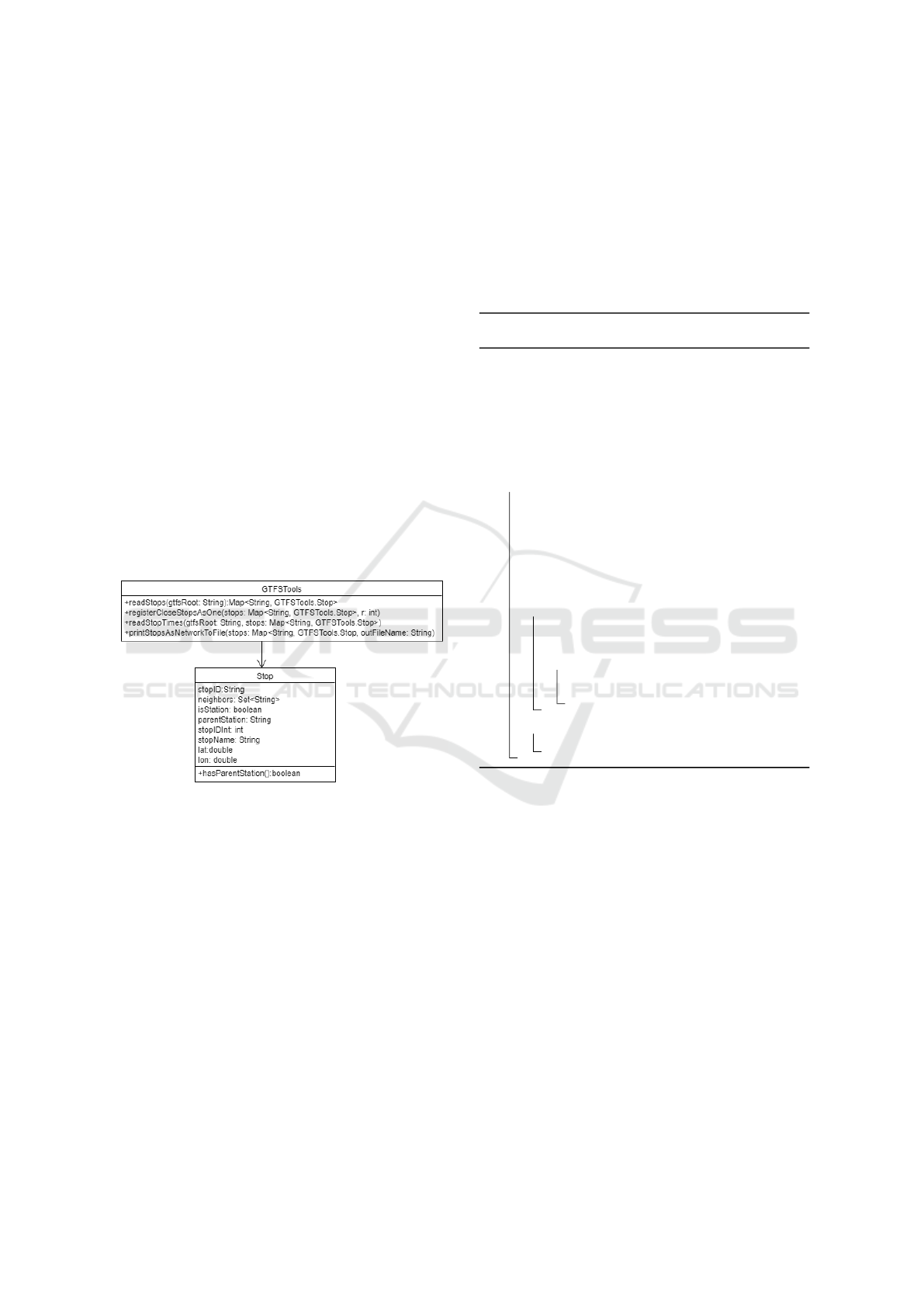
Figure 2: The UML class diagram of the network converter

tool. The Stop class is an inner class of GTFSTools.

One can note on Figure 2 that the GTFSTools

class has 4 public methods. readStops(...) builds

the nodes of the network, readStopTimes(...)

connects them (or the parent stations of them) by

edges, while printStopsAsNetworkToFile(...)

prepares the exported network ﬁle. The

registerCloseStopsAsOne(...) method is

needed to be called only if one would like to merge

stops close to each other to one. If this is needed it

has to be called just before the readStopTimes(...)

method. The r: int parameter of this latter method

speciﬁes the merging distance below which we accept

two stops to be merged.

It has to be mentioned that ﬁnding the close stops

in a set of stops is not a trivial problem especially if

we try to take care on the efﬁciency aspects. Finally

in our solution we have used the recursive algorithm

described in Alg. 1. Note that what we have imple-

mented is at the background a one dimensional Sur-

rounding Cell Registration algorithm (Ogami, 2021)

where we ﬁrst ﬁnd the close stops according to the

longitudinal distances and then keep only those from

the potential close stops whose Haversine distance is

small enough (smaller or equal to r).

Algorithm 1: Algorithm to merge close stops by virtual sta-

tions.

Input: Set of stops and parent stations, r

Output: Set of stops and virtual parent

stations

1 Copy the stops (their references) to a sorted

list stops. (Sorted by the longitudinal

position of them)

2 actIdx=0, bottomIdx=0, topIdx=0

3 for actIdx ∈ 0..stops.size do

4 bottomIdx=the ﬁrst stop’s index in the list

for which stops[botomIdx].lonPos >

stops[actIdx].lonpos-r

5 topIdx=the last stop’s index in the list for

which stops[topIdx].lonPos <

stops[actIdx].lonpos+r

6 for idx ∈ bottomIdx..topIdx do

7 if

distance(stops[idx],stops[actIdx])<r

then

8 Add stops[idx] to the set of close

stops

9 for each stop in the list of close stops do

10 repeat steps 4, 5, 6

A natural outcome of this algorithm is that by in-

creasing the value of the checked distance r, we get

less nodes in our resulted network. An interesting

question is that what may be a reasonable value for

r in order not to loose too many stops but still elimi-

nate the cases when e.g. stops at two sides of the same

road are handled as being independent (since maybe

no common parent station has been added to them).

In order to be able to give a hint how to select

the value of r we have checked the dependence of

the number of nodes N on the distance r for several

GTFS feeds (A detailed description of each feed and

the sources of them are available at the GitHub of the

project’s data (Kocsis and Varga, 2021b)).

Our ﬁndings are summed up on Figure 3. As one

may observe increasing the merging distance r at the

ﬁrst some meters does not affect much the number of

stops since it is really rare that there are two inde-

pendent stops this close (without being two stops of

COMPLEXIS 2022 - 7th International Conference on Complexity, Future Information Systems and Risk

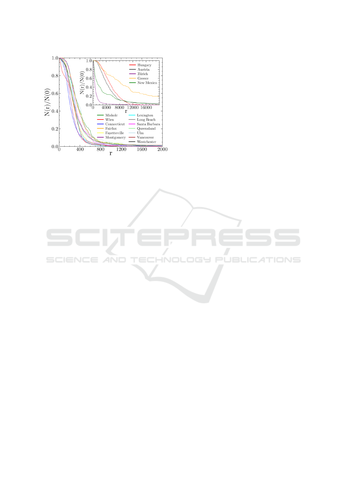
Figure 3: Normalized number of nodes N

in the net-

work as a function of the merging distance r. Note that

for most feeds a strong decrease starts around r = 100m or

r = 200m. Inset: non-local transport network cases on a

longer scale. See detailed description of the data at (Kocsis

and Varga, 2021b).

a station). As the trends show in most cases however

somewhere around 100 − 200 meters the number of

stops N starts to fall down rapidly showing that this

distance may be the desired one describing close sta-

tions that may be merged in order to see a more valid

picture of the network of mass transportation systems.

This ﬁnding is consistent to the intuitive guess

based on studying mass transportation maps, that the

distance of such stations should be somewhere around

150 meters. The exact value however is to be decided

based on the actual data since special local properties

may affect it.

One may also note on Figure 3 that while most of

the curves move together following an inverse logistic

shape, there are some of them that seem to have dif-

ferent behavior. Examining these cases however soon

reveals that these exceptional cases are for transporta-

tion feeds describing non-local or non-exclusively-

local transportation networks, like train, ferry and

inter-city bus networks. Nevertheless drawing these

data on a longer scale shows that their qualitative be-

havior do not differ (see Figure 3 inset). We see simi-

lar falling of the curves as before for these cases as

well, just the place of it is around 2-4 kilometers.

It has to be noted however that merging stops more

than 2 kilometers far from each other may not have

any practical use especially knowing that luckily in

the case of train stations it is really rare that compa-

nies register the two directions as individual stops (not

even grouped by a parent station).

5 INVESTIGATION OF SOME

RESULTED NETWORKS

In order to see how our tool works on extracting net-

works from GTFS feeds in practice we have used it

for several transportation feeds available online. We

have collected these sources under the GitHub page

of our project (Kocsis and Varga, 2021a), (Kocsis and

Varga, 2021b) and also we have uploaded there the re-

sulted abstract networks in .txt format. A conclud-

ing table of these extracted networks together with

some basic properties of them are shown on Figure

4. Note that there are huge differences in the number

of nodes of the networks for different sources. Some

service providers have only a bit more than 100 nodes,

while some of them have ten-thousands.

In most of the cases the union of close nodes

(merging stops within r = 150m distance by virtual

parent stations) decreases the number of nodes al-

most to the half of the original node number in case

of r = 0m. This conﬁrms the assumption that stops

at the opposite side of roads, or being close to each

other in different ways are quite frequent in the source

data sets (note again the position of bus stops on the

real map shown on Figure 1). These related stops

are handled independently by most of the GTFS feeds

however from the passengers’ point of view they usu-

ally mean the same location during their journey on

the urban public transport system. Contrarily, there

are some systems (like New York City subway or the

Hungarian train system e.g.) that are almost unaf-

fected by our algorithm, namely the merging process

does not change too much the number of nodes (in

case of r = 150). These are however mainly railway

systems, where the opposite direction trafﬁc use the

same platform or if there are multiple platforms, they

are contained by parent stations already in the original

transportation feed.

Some extracted networks in case of r = 0m con-

tain only one cluster of nodes, meaning that all the

nodes are available from any nodes via a link se-

quence. This practically means that passengers can

travel from a stop to any other by the given public

transport system. Nevertheless a signiﬁcant portion of

the analyzed systems fall apart several isolated clus-

ters, where there is no connection at all between the

nodes of these separate clusters. It seems strange if

a public transport systems does not provide any ser-

vice to connect different regions, but we will see that

usually this is just a side effect of the missing parent

stations of close stops. Usually but not exclusively

one of these clusters is much larger then others, so

beside the giant cluster there are several minor clus-

ters of stops and stations.

Extracting Mass Transportation Networks from General Transit Feed Speciﬁcation Datasets

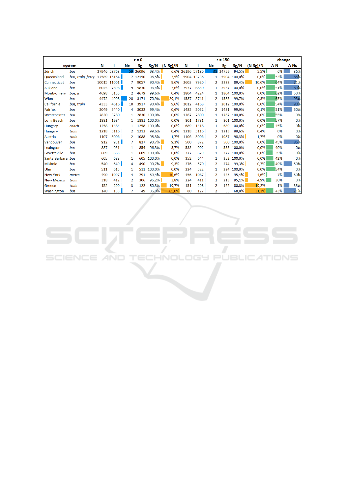
Figure 4: Basic properties of networks extracted from some example GTFS feeds for merging distance r = 0m and r = 150m.

Note the huge level of change implied as a result of merging close stops (see the last two columns). N: number of nodes in

the network, L: number of edges in the network, N

: number of clusters, S

: size of the giant cluster.

Our algorithm can transform this network by the

merging of near stops to create a new virtual station.

Our results show that using r = 150m distance im-

plies that almost all networks compose only one or

two clusters. For a passenger this means that a few

steps long walk can dramatically improve the connec-

tivity of the network. It should be mentioned, that the

only exception is the GTFS feed of Z

urich, where the

service provider operates services not exclusively in

urich, but in further places as well resulting in small

independent clusters. The numerical results can be

seen on Figure 4.

6 CONCLUSIONS

In this paper we have given a basic introduction to

the structure of General Transit Feed Speciﬁcation

highlighting the most important properties of it from

the aspect of extracting a network of connected stops

from the source feeds. Besides describing the process

we have even implemented the extraction in a free to

use tool.

We have put a special focus on the use (or not

use) of parent stations in GTFS feeds. As a possi-

ble solution to handle the problem of close stops in

the extracted networks we used the merging distance

r to describe how close stops are to be handled as be-

ing stops of the same so called ‘’virtual station”. In

some example networks extracted from various GTFS

feeds we have investigated the effect of increasing r.

We have found that the intuitive value of r = 150m

is a reasonable choice also from the aspect of our nu-

merical investigations. We have presented some basic

properties of these networks at the end.

Our ongoing research now has a focus on the use

of the tool providing more mass-transportation net-

works to be used by other scientists (with the descrip-

tion of these networks). Integrating the API of Open-

MobilityData would be e.g. a very useful extension.

We also plan to further upgrade the tool to make the

extracted network depend on more parameters. And

also we would like to provide a simple Graphical User

Interface to make the tool even more easy to be used.

We have found that building a web service for this aim

would not be worthy.

ACKNOWLEDGEMENTS

This work was supported by the EFOP-3.6.1-16-

2016-00022 project.

The project is co-ﬁnanced by the European Union and

the European Social Fund.

COMPLEXIS 2022 - 7th International Conference on Complexity, Future Information Systems and Risk

REFERENCES

Besenczi, R., B

atfai, N., Jeszenszky, P., Major, R., Monori,

F., and Isp

any, M. (2021). Large-scale simulation

of trafﬁc ﬂow using markov model. PLOS ONE,

16(2):e0246062.

Braga, M., Santos, M. Y., and Moreira, A. (2014). New

Perspectives in Information Systems and Technolo-

gies, chapter Integrating Public Transportation Data:

Creation and Editing of GTFS Data, pages 53–62.

Springer.

Fortin, P., Morency, C., and Tr

epanier, M. (2016). Inno-

vative gtfs data application for transit network analy-

sis using a graph-oriented method. Journal of Public

Transportation, 19(4).

Gallotti, R. and Barthelemy, M. (2015). The multilayer tem-

poral network of public transport in great britain. Sci-

entiﬁc Data, 2:140056.

Hansson, J., Pettersson, F., Svensson, H., and Wretstrand,

A. (2019). Preferences in regional public transport: a

literature review. European Transport Research Re-

view, 11:38.

Harrelson, C. (2021). GTFS Reference. Google.

https://developers.google.com/transit/gtfs.

Jiang, B. (2007). A topological pattern of urban street net-

works: Universality and peculiarity. Physica A: Sta-

tistical Mechanics and its Applications, 384:647–655.

Real city map topology, trafﬁc information (80scale-

free.

Kocsis, G. and Varga, I. (2021a). Github page of the project.

https://github.com/kocsisger/gtfs2net.

Kocsis, G. and Varga, I. (2021b). Github page of the used

gtfs feeds. https://github.com/kocsisger/gtfs.

Kujala, R., Weckstr

om, C., Darst, R. K., Mladenovi

M. N., and Saram

aki, J. (2018a). A collection of pub-

lic transport network data sets for 25 cities. Scientiﬁc

Data, 5:180089. GTFS network collections of cities,.

Kujala, R., Weckstr

om, C., Darst, R. K., Mladenovi

M. N., and Saram

aki, J. (2018b). A collection of pub-

lic transport network data sets for 25 cities. Scientiﬁc

Data, 5(180089).

ammer, S., Gehlsen, B., and Helbing, D. (2006). Scaling

laws in the spatial structure of urban road networks.

Physica A: Statistical Mechanics and its Applications,

363:89–95. 20 german cities road network, distribu-

tion of cars on roads.

Ogami, Y. (2021). Fast algorithms for particle searching

and positioning by cell registration and area compar-

ison. Trends in Computer Science and Information

Technology, 007-016(6(1)).

Porta, S., Crucitti, P., and Latora, V. (2006). The network

analysis of urban streets: A dual approach. Physica A,

369:853–866. Complex network of roads of 6 cities,

node-edge swapping representation, maps, P(k), acc,

avk, apl.

Rosetta Code Community (2021). Haversine formula.

https://rosettacode.org/wiki/Haversine formula.

Sienkiewicz, J. and Hołyst, J. A. (2005). Statistical analysis

of 22 public transport networks in poland. Physical

Review E, 72:046127.

von Ferber, C., Holovatch, T., Holovatch, Y., and

Palchykov, V. (2007). Network harness: Metropolis

public transport. Physica A: Statistical Mechanics and

its Applications, 380:585–591.

Vuurstaek, J., Cich, G., Knapen, L., Ectors, W., Yasar, A.-

U.-H., Bellemans, T., and Janssens, D. (2020). Gtfs

bus stop mapping to the osm network. Future Gener-

ation Computer Systems, 110:393–406.

Wessel, N. and Farber, S. (2019). On the accuracy of

schedule-based gtfs for measuring accessibility. Jour-

nal of Transport and Land Use, 12(1):475–500.

Wong, J. C. (2013). Use of the general transit feed speci-

ﬁcation (GTFS) in transit performance measurement.

PhD thesis, Georgia Institute of Technology.

Extracting Mass Transportation Networks from General Transit Feed Speciﬁcation Datasets