Scalable Infrastructure for Workload Characterization of Cluster Traces

Thomas van Loo

, Anshul Jindal

1 a

, Shajulin Benedict

2 b

, Mohak Chadha

1 c

and Michael Gerndt

1 d

Chair of Computer Architecture and Parallel Systems, Technical University Munich, Germany

Indian Institute of Information Technology Kottayam, Kerala, India

Keywords:

Cloud Computing, Google Cloud, Scalable, Workload Characterization, Google Cluster Traces, Dataproc.

Abstract:

In the recent past, characterizing workloads has been attempted to gain a foothold in the emerging serverless

cloud market, especially in the large production cloud clusters of Google, AWS, and so forth. While analyzing

and characterizing real workloads from a large production cloud cluster beneﬁts cloud providers, researchers,

and daily users, analyzing the workload traces of these clusters has been an arduous task due to the heteroge-

neous nature of data. This article proposes a scalable infrastructure based on Google’s dataproc for analyzing

the workload traces of cloud environments. We evaluated the functioning of the proposed infrastructure us-

ing the workload traces of Google cloud cluster-usage-traces-v3. We perform the workload characterization

on this dataset, focusing on the heterogeneity of the workload, the variations in job durations, aspects of re-

sources consumption, and the overall availability of resources provided by the cluster. The ﬁndings reported in

the paper will be beneﬁcial for cloud infrastructure providers and users while managing the cloud computing

resources, especially serverless platforms.

1 INTRODUCTION

In an attempt to invade the minds of cost-conscious

users, the cloud providers constantly launch newer ex-

ecution models or approaches such as “serverless“ to

reduce the cost involved in many applications, espe-

cially IoT-enabled applications (Carreira et al., 2019).

There is a shift in the utilization of cloud comput-

ing resources such as VMs, monolithic services, mi-

croservices, and serverless (Fan. et al., 2020). This

evolves into varying cloud workloads with complex

resource characteristics and requirements for cloud

application developers or infrastructure providers.

Cloud workloads, in general, are classiﬁed into

two broad classes: i) production jobs that are often

latency-sensitive and highly available, and ii) non-

production batch jobs that are short-lived and less

performance-sensitive jobs (Alam et al., 2015). These

workloads need to be diligently assessed for the bet-

ter utilization of cloud resources or for enabling a

cost-efﬁcient framework. In fact, to achieve cost ef-

ﬁciency, scalability, energy efﬁciency, and so forth, a

https://orcid.org/0000-0002-7773-5342

https://orcid.org/0000-0002-2543-2710

https://orcid.org/0000-0002-1995-7166

https://orcid.org/0000-0002-3210-5048

few approaches were practiced in the past by cloud

infrastructure providers. For instance, approaches

such as co-locating suitable serverless functions in the

form of establishing a fusion of functions (Elgamal

et al., 2018), identifying appropriate cloud resources

for computations (Espe. et al., 2020), monitoring the

behavior of underneath infrastructures (Chadha et al.,

2021), and so forth, have been practiced in the past.

Identifying appropriate cloud resources, in gen-

eral, requires a diligent understanding of the exist-

ing workloads and their characteristics. However,

there are a few challenges for realizing a better per-

formance in the cloud due to the timely characteri-

zation of workloads, especially in the evolving cloud

markets. A few notable challenges include:

1. non-availability of the real-workload traces to pre-

dict the resource utilization pattern of clouds;

2. delayed characterization of workloads;

3. increasing heterogeneity of resources and work-

loads – e.g., FaaS clusters established using Rasp-

berry Pi require minimal computational capabil-

ities when compared to compute clusters estab-

lished using VMs; and, so forth.

Analyzing the cloud workloads beneﬁts the efﬁcient

utilization of cloud resources; besides, it can also

254

van Loo, T., Jindal, A., Benedict, S., Chadha, M. and Gerndt, M.

Scalable Infrastructure for Workload Characterization of Cluster Traces.

DOI: 10.5220/0011080300003200

In Proceedings of the 12th International Conference on Cloud Computing and Services Science (CLOSER 2022), pages 254-263

ISBN: 978-989-758-570-8; ISSN: 2184-5042

lead to effective provisioning of the available het-

erogeneous compute nodes (Perennou et al., 2019).

Accordingly, leading cloud providers delivered their

workload traces for further workload characteriza-

tion and analysis – i.e., Google exposed the traces

of workloads carried out at the Borgs’ workload

for analyzing the cloud resources (Wilkes, 2011;

Wilkes, 2020a; Wilkes, 2020b); Microsoft’s Azure

constantly updated the traces of its workloads for re-

searchers (Cortez et al., 2017); Alibaba distributed

the CPU utilization of VM workloads of its data-

center (Guo et al., 2019); and, so forth. Although

traces are available for further analysis and actions,

the existing methods are either not capable of han-

dling larger data traces or inappropriate to handle the

heterogeneous nature of workloads.

In this article, a scalable workload characteriza-

tion infrastructure based on Google’s “Dataproc“ is

proposed (GoogleCloud, 2016b). The infrastructure

is laid on a spark-based cluster such that the BigQuery

clients of the architecture analyze the real workload

traces of clouds. Experiments were carried out us-

ing Google cluster-usage traces v3 at our estab-

lished scalable infrastructure (Wilkes, 2020a; Wilkes,

2020b). In addition, the traces were analyzed from

three perspectives: i) analyzing the heterogeneity of

the workload traces of the Borg’s cluster; ii) charac-

terizing the long or short cloud workloads; evaluating

the resource consumption of tasks; and, iii) examin-

ing the utilization of cloud resources.

Paper Organization: Section 2 discusses the exist-

ing research works in the workload characterization

domain; Section 3 explains the details of the proposed

scalable architecture; Section 4 illustrates the experi-

mental results and associated discussions; and, ﬁnally,

Section 5 expresses a few outlooks on the work.

2 RELATED WORK

Cloud has remarkably marked its footprints in several

research domains, surpassing from IoT to HPC do-

mains (Carreira et al., 2019). A few research works

have been practiced in the past to effectively utilize

the cloud resources for varying domains in datacen-

ters and industrial cloud infrastructures. Character-

izing cloud workloads has been considered to bene-

ﬁt cloud providers/users due to the cost-effective uti-

lization of resources (Kunde and Mukherjee, 2015;

Pacheco-Sanchez et al., 2011). Since the ﬁrst re-

lease of the workload trace of a Borg cluster in

2010 (Hellerstein, 2010), the cloud community has

endeavored to inspect the cloud workload traces in

varied fashions to reap in the ultimate insights of the

clouds and workload distributions.

Researchers in the past have analyzed a month-

long trace of the single cluster in Google’s Borg to

study the heterogeneity and dynamicity of the work-

loads (Reiss et al., 2012; Rasheduzzaman et al., 2014;

Minet et al., 2018). Authors of (Reiss et al., 2012)

studied the challenges due to the inclusion of hetero-

geneous workloads and inefﬁcient resource schedul-

ing aspects of cloud resources. A few authors at-

tempted to apply machine learning algorithms to as-

sess the workloads of traces. For instance, the authors

of (Alam et al., 2015) and (Gao et al., 2020) have uti-

lized the data traces to predict the workload require-

ments when executed on the cloud environments. The

authors clustered the cloud workloads of similar pat-

terns after developing a machine learning model.

The dataset, we analyze in this work (Wilkes,

2020a; Wilkes, 2020b), was released in April 2020.

The main addition to the third google cluster trace

compared to the second was the tracing of 8 separate

clusters spread out through North America, Europe,

and Asia instead of the measurements of a single clus-

ter as provided in the second trace. Furthermore, three

additions have been made to the properties recorded:

CPU usage information histograms are provided ev-

ery 5 minutes instead of the previous single point

sample. Alloc sets were equally introduced to the

third trace, which was not present in the 2011 dataset.

Lastly, job-parent information for master/worker re-

lationships, such as MapReduce, has been added. It

is also worth noting that at approximately 2.4TiB of

data, this trace is far more signiﬁcant than the previ-

ous recordings. Due to its size, the third trace has only

been made publicly available in Google’s cloud data

warehouse, BigQuery (GoogleCloud, 2016a).

In previously existing approaches, the analysis has

been executed on a single machine or has not con-

sidered the recent cloud data traces. Thus, this work

proposed the scalable workload characterization envi-

ronment to evaluate the cloud workloads.

3 INFRASTRUCTURE

To handle large volume of cloud workload traces and

analyze the characteristics of them, we proposed a

scalable environment consisting of Dataproc

from

the Google cloud. The proposed scalable infrastruc-

ture paved way for efﬁcient data analytics processing

much faster than the other approaches. A high level

overview of the proposed infrastructure and work-

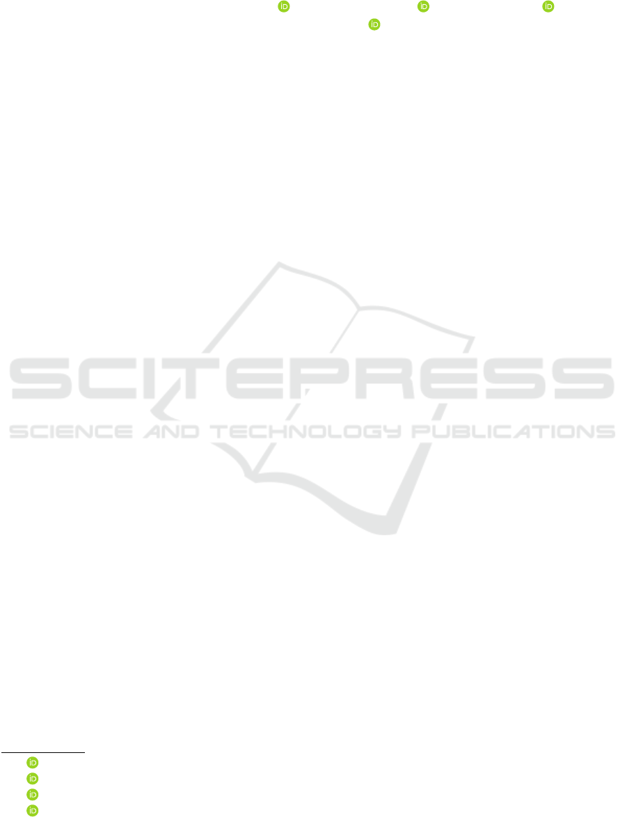
ﬂow is shown in Figure 1. The important entities

https://cloud.google.com/dataproc

Scalable Infrastructure for Workload Characterization of Cluster Traces

255

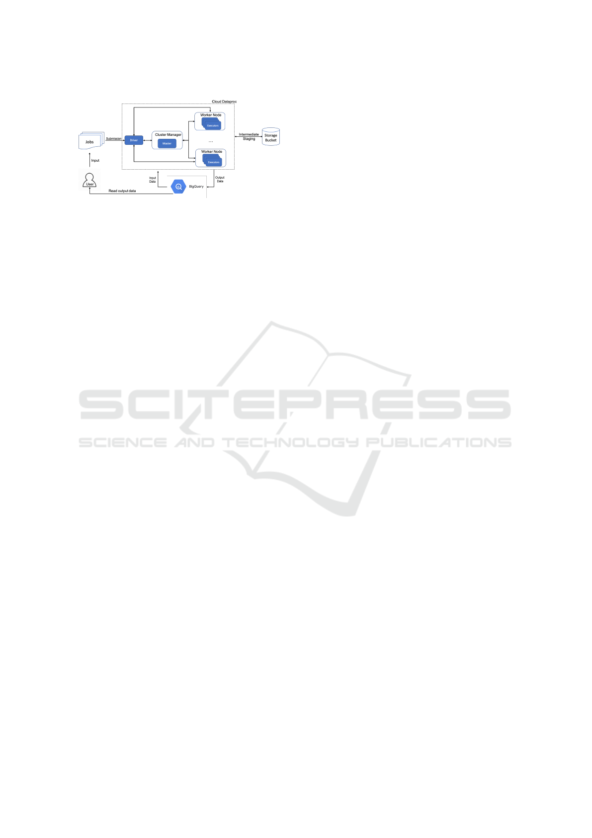
Figure 1: Scalable Infrastructure based on Google Cloud

Dataproc for Workload Characterization.

that are available in the proposed scalable architecture

and their functionalities are described in the following

subsections.

3.1 YARN-Cluster

To cope with the evolving range of cloud workload

traces, we included Yet Another Resource Negotia-

tor (YARN) cluster in the architecture using Google’s

“Dataproc“ component. YARN, in general, can han-

dle big data for analytics purposes. It is lightweight

due to the metadata model of establishing clusters.

Firstly, a YARN (Yet Another Resource Negotiator)

based spark cluster is created using the Dataproc.

This cluster consists of one master node and “n“

worker nodes, where n is equal or greater than 2. The

master node manages the cluster, creating multiple

executors within the worker nodes. These executors

are responsible for running the tasks in parallel. The

type of the virtual machine used for the master and

worker nodes can be speciﬁed along with the nec-

essary libraries required for the job while creating a

cluster. Once the cluster is created, the libraries are

installed automatically and are conﬁgured to be linked

with external Storage Units which the executors use.

3.2 Storage Units

The proposed scalable architecture includes external

storage units – e.g., google cloud storage buckets – for

processing the workload traces. These storage units

are responsible for performing intermediate data stag-

ing while executing the tasks. In most cases, these are

required for executing the analysis tasks.

3.3 Job Submissions

Analyzing cloud workload traces is carried out by

submitting the jobs to the scalable infrastructures via

the job submission portal. The Job Submission por-

tal is designed using PySpark or Spark-based job de-

scription system connected with the BigQuery com-

ponent. The primary purpose of including the Big-

Query component in the system is to enable the ex-

ecutors to access data directly from the BigQuery. In

doing so, the users could view or utilize the envi-

ronment to further process traces. Additionally, the

Job Submission portal is designed to establish an au-

toscaling feature of worker nodes to make the analysis

of workloads scalable.

3.4 Dataset Access

A more appropriate dataset with suitable cloud work-

load information is crucial for characterizing the

cloud jobs. The proposed scalable architecture ap-

plied the most recent Google Cluster-Usage traces

v3 for the characterization of the clouds. Access-

ing cloud traces in the proposed scalable architecture

is handled through the BigQuery-based serverless

platform. In general, BigQuery is a fully-managed,

serverless data warehouse that enables scalable, cost-

effective and fast analysis over petabytes of data. It

is a serverless Software-as-a-Service (SaaS) that uses

standard SQL by default as an interface (Google-

Cloud, 2016a). It also has built-in machine learn-

ing capabilities for analyzing the dataset capabilities.

There are various available methods to access data

within BigQuery, including a cloud console, a com-

mand line tool and a REST API. In this work, we pre-

ferred BigQuery API client library based on Python

due to the inherent capabilities of processing machine

learning features.

4 RESULTS

In this section, we ﬁrst discuss the workload charac-

terization from four different aspects: i) Heterogene-

ity of collections and instances (§4.1), ii) Jobs’ dura-

tion characterization (§4.2), iii) Tasks’ resources us-

age (§4.3), and iv) Overall cluster usage (§4.4).

4.1 Heterogeneity of Properties

This part of the analysis is focused on the hetero-

geneity of the properties within the CollectionEvents

and InstanceEvents tables, as well as examining and

visualizing the quality of the dataset. We will go

property by property, commencing with those that are

common within both tables (§4.1.1), then the ones

speciﬁc to CollectionEvents (§4.1.2) and lastly spe-

ciﬁc to InstanceEvents (§4.1.3).

CLOSER 2022 - 12th International Conference on Cloud Computing and Services Science

256

Table 1: Occurrences of collection scheduling classes.

Tier Percentage of all jobs

Free 1.6%

Best-effort Batch 9.1%

Mid 3.8%

Production 85.2%

Monitoring 0.3%

4.1.1 Common Properties

We begin by examining the total amount of collec-

tions and instances submitted throughout the trace pe-

riod to gain a broader overview of the spectrum of the

tables. There are a total of approximately 20.1 mil-

lion rows in the CollectionEvents table, which rep-

resent events that occur on the roughly 5.2 million

unique collection id’s present. Over 99% of these

are jobs, with roughly 36 thousand alloc sets. The

InstanceEvents table comprises roughly 1.7 billion

rows, which represent the number of instances spread

out over the 5.2 million collections. Approximately

87% of the instances are tasks and roughly 13% alloc

instances. We further investigate the distribution of

the occurrences of the different event types through-

out the dataset. The count for each type in the table is

displayed in Figure 2a.

From Figure 2a we can see that, the most common

events are SUBMIT, ENABLE, SCHEDULE, FINISH

and KILL which were to be expected. As an additional

step, we count the number of collection events that

are associated with these events per day (excluding

ENABLE as this is comparable to SCHEDULE in this

context). Figure 3a shows the result. We ﬁnd from the

result that: (1) the number of scheduled collections

shows a certain periodicity to an extent as every 14

days, the count falls for several days. (2) Collections

are frequently killed, far more often than they ﬁnish

normally. (3) During the last nine days of the trace,

there was a surge of activity, with almost double the

amount of submitted and scheduled collections.

Collections and instances are equipped with a pri-

ority property: a small integer, with higher values in-

dicating higher priorities. Those with more signiﬁ-

cant priorities are given preference for resources over

those with smaller priorities. The values can be sub-

categorized into 5 tiers and the distribution of jobs

within these 5 tiers is shown in Table 1, with the pro-

duction tier as the clear majority.

As with the event types, we display the number

of events associated with each priority tier for each

day. We can see in Figure 3b, the production and

best-effort batch tier jobs follow the same trends as

the event types throughout the trace, contrary to the

free, mid, and monitoring tier jobs, which show no

Table 2: Occurrences of max per machine values.

Max per Machine Count

1 35150

2 289

10 2

25 36

discernible patterns.

The last property common to both tables is alloc -

collection id, the id of the alloc set that hosts the job,

or empty if it is a top-level collection. Upon inves-

tigating this property, we found roughly 97.7% of

jobs to be top-level collections and a mere 0.3% to

be hosted by alloc sets.

4.1.2 CollectionEvents – Speciﬁc Properties

The ﬁrst property we examine that is unique to Col-

lectionEvents is parent collection id, the ID of the

collection’s parent or an empty value if it has none.

We found that approximately 64% of all collections

had parent ID, indicating that most collections are re-

lated to others.

The next distribution we investigate is that of the

max per machine, the maximum number of instances

from a collection that may run on the same machine.

About 99% of all collections do not have a constraint

in this regard. For the remaining 1% with a max -

per machine value, there are four unique values that

exist in the table. These values and their counts are

displayed in Table 2.

From these occurrences, we can see that should a

collection come with a constraint for instances run-

ning on a single machine, around 99% of the time, it

will be limited to 1 instance per machine. Similar to

the previous property, max per switch displayed sim-

ilar tendencies, with over 99% of collections not hav-

ing any constraints. The few that had a value for this

ﬁeld amounted to 21 unique values ranging from 1

to 104. 99% of these collections were limited to one

instance per switch.

Users have the option of enabling vertical scal-

ing when submitting a job, allowing the system to de-

cide how many resources are required autonomously.

The dataset displays this information via four unique

values in this ﬁeld. Table 3 shows the result of the

examination of the distribution of the values for ver-

tical scaling. We see that most users have enabled

vertical scaling, most of which are bound by user-

speciﬁc constraints. We assume the constraints are

widely used to ensure cost-effectiveness when con-

suming cloud resources.

Scalable Infrastructure for Workload Characterization of Cluster Traces

257

(a) CollectionEvents table. (b) InstanceEvents table.

Figure 2: Number of occurrences of different event types within two major types of tables.

(a) Occurrences of SUBMIT, SCHEDULE, FINISH and

KILL events in CollectionEvents per day.

(b) Counts of events associated with the 5 priority tiers per

day.

Figure 3: Occurrences of events during the course of trace collection time.

Table 3: Distribution of values for vetical scaling.

vertical scaling value Percentage of Jobs

Setting Unknown 0.0%

Off 6.8%

User-Constrained 66.6%

Fully Automated 26.6%

Table 4: Distribution of job sizes in terms of tasks per job.

Number of Tasks Number of Jobs

1 4,067,109

2 - 10 906,736

11 - 100 149,516

101 - 1000 72,984

1001 - 2000 7,715

> 2000 9,606

4.1.3 InstanceEvents – Speciﬁc Properties

We begin the InstanceEvents speciﬁc properties by

analyzing the instance index column, which indicates

the position of an instance within its collection. Us-

ing this information, we can determine variations in

the number of tasks within jobs. The maximum value

in the table for this ﬁeld is 97,088. In Table 4, we dis-

play the job size distribution in terms of tasks per job,

separated into 6 bins. We can see that jobs primarily

have several tasks under ten and rarely over 1000.

Furthermore, we examine the machine id property

that provides the ID of the machine an instance was

scheduled on. We found that roughly 51.9% of all

instances had been scheduled on a machine, while the

remaining 48.1% are yet to be scheduled.

4.2 Job Duration Characterization

In this section, we ﬁrst discuss the overall characteri-

zation of short and long job’s durations and their suc-

cess rates (§4.2.1). Then we analyze the jobs’ dura-

tions and success rates by priority tier (§4.2.2). Lastly,

we analyze the variations of time spent in different

states of a jobs’ lifecycle (§4.2.3).

4.2.1 Overall Jobs’ Durations and Success Rates

We measure job durations in seconds, the longest

possible duration in the dataset being around

2,600,000s seconds (30 Days). Further, we found

that roughly 85.3% of all jobs had a duration between

0s and 1000s, only around 0.4% run longer than one

day, and a total of 48 jobs runs during the entire trace

period. Of the jobs that ran under 1000s, around 60%

had a run time under 100s, which is around half of

the jobs.

4.2.2 Jobs’ Durations & Success Rates by

Priority

In this section, we analyze the jobs’ durations and

their success rates by priority tiers. The success rates

of jobs in all the tiers is shown in Table 5.

CLOSER 2022 - 12th International Conference on Cloud Computing and Services Science

258

Table 5: Success rates of jobs in all the tiers.

Final State Free BEB Mid Prod. Monit.

KILL 49.2% 58.9% 49.5% 76.5% 9.2%

FINISH 47.4% 36.9% 48.9% 23.1% 4.4%

FAIL 3.4% 4.2% 1.6% 0.4% 81.3%

SCHEDULE 5.1%

Free Tier: The overall jobs’ durations distribution

is analogous to the overall distribution, with the run

times under, 1000s and the majority of those jobs run

under 100. From Table 5, we see that the kill to ﬁn-

ish ratio is more balanced here, being almost equally

distributed.

Best-effort Batch Tier: They showed slightly ele-

vated levels of jobs that ran longer than 1000s in com-

parison to the overall distribution, yet had no jobs

running longer than a day. This is to be expected,

as best-effort batch tier was conceived for jobs han-

dled by the batch scheduler. The mean run time for

best-effort batch tier is roughly 7227s. From Ta-

ble 5, we observe that the success rates for best-effort

batch tier are less evenly spread in comparison to the

free tier, with a higher KILL rate. This suggests that

longer running jobs could be killed more frequently

than shorter running ones.

Mid Tier: They also displayed a similar run time dis-

tribution as the overall one, except having a slightly

more elevated count of jobs that lasted between 1000s

and 2000s. The mean job duration within this cat-

egory is approximately 6653s. From Table 5, the

success rate is evenly distributed among FINISH and

KILL, a further indication that longer jobs tend to be

killed more often than shorter ones.

Production Tier: They displayed a very similar pat-

tern to the overall free and mid tier distributions, con-

sisting heavily of jobs with runtimes under 1000s and

having a mean of about 1885s. This indicates that

production jobs, which have the highest priority for

everyday use, mainly consist of short-running jobs

that ran under 100s. From Table 5, contradictory to

our previous assumption, production jobs show an ap-

parent tendency to be killed more frequently than not,

despite consisting almost exclusively of very short-

running jobs.

Monitoring Tier: As expected, with a mean of

42,970s, the runtimes of jobs in the monitoring tier

are, on average, the longest of all tiers. The large ma-

jority of them ran between 3000s and 4000s, but this

group was also the only one with visible counts for

runtimes over 50,000s seconds. The success rate for

this tier, shown in table 5, is characterized by a re-

sounding majority of jobs failing, a clear indication

that long-running jobs have a much higher tendency

to fail than shorter ones. Some jobs last state were

also recorded as SCHEDULE. We expect these jobs

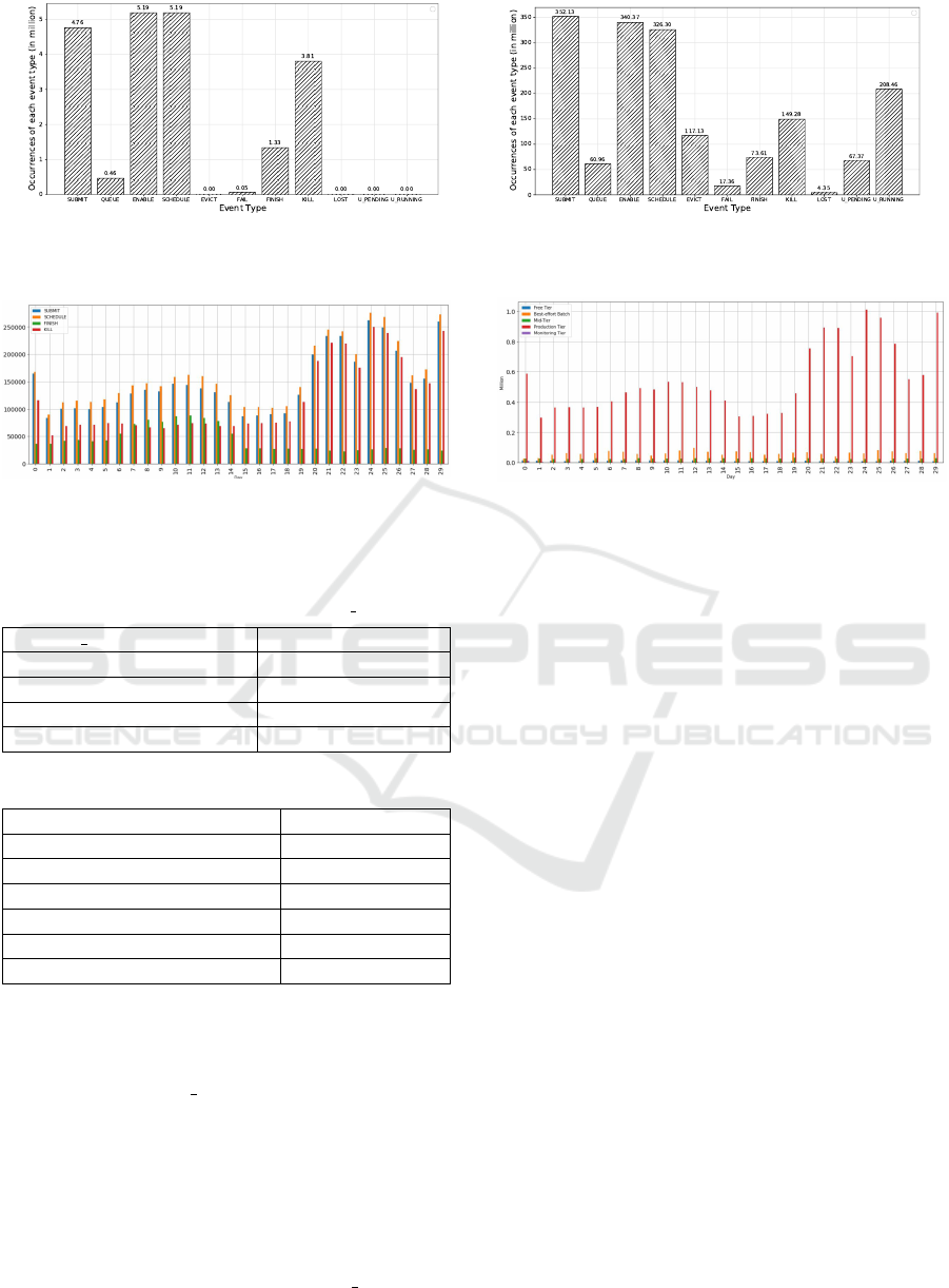
Figure 4: Mean durations of jobs spent in each state.

ran during the entire trace period without ﬁnishing.

4.2.3 Job State Durations

This section analyzes the time spent by jobs in dif-

ferent states, speciﬁcally SUBMIT, QUEUE, EN-

ABLE, SCHEDULE, UPDATE RUNNING and UP-

DATE PENDING. The other four states mark the end

of a job’s life cycle and do not have a duration. We

do this by examining these six states’ mean. It is

to be noted that these events are not actually states,

but events that trigger transitions between job states;

however, by determining the elapsed time between

these transitions, we can calculate how much time

was spent in the respective state. For this reason, we

refer to these events as states in this section.

Figure 4 shows the mean durations of jobs spent in

each state. With around 424,477s, UPDATE RUN-

NING is the state with the most extended value by a

large margin. The mean values for the other states

are barely visible in the comparison graph. We, there-

fore, display the graph without the value for UPDATE

RUNNING in Figure 4, allowing a more apt compari-

son. This state also had the lowest occurrence, having

only a count of 20 jobs that ran an update during the

trace. Though updates rarely happen, we can con-

clude that they tend to be much more time costly.

From Figure 4, we further see that the second-

highest value is for the QUEUE state. Upon further

investigation, we found that the majority of jobs spent

under 100s in this state, yet numerous outliers are

ranging from over 1000s till a maximum of around

1,200,000s, which explains the higher mean value.

We suspect these are jobs in the lower priority tiers

that have to remain in queue until higher priority jobs

yield compute resources to run on.

From the three remaining states, we conclude that:

(1) The time lapses between a job being SUBMIT-

TED and either ENABLED or QUEUED is relatively

low, which shows the time between submission and

eligibility to be scheduled is kept at a minimum. (2)

The low mean of ENABLE state signiﬁes that once a

job becomes eligible for scheduling, it does not take

long for the scheduler to place it compared to the rest

of the job’s life cycle. (3) When a job needs to be

updated, the pending time before the update is per-

Scalable Infrastructure for Workload Characterization of Cluster Traces

259

(a) Requested. (b) Consumed.

Figure 5: Average CPU and memory requested and consumed per day.

formed is meager, unlike the average update time.

4.3 Task Resource Usage

In this section, we ﬁrst analyze the amount of re-

sources that are requested by tasks, which is saved in

the resource request column of the InstanceEvents

table as a structure (§4.3.1). It represents the maxi-

mum CPU or memory a task is permitted to use. Sec-

ond, we analyze the amount of resources consumed

by tasks, which is recorded in the InstanceUsage ta-

ble (§4.3.2). These two aspects can then be compared

to view the general resource requirements for a clus-

ter to handle this type of workload and see if tasks

resource limits are adhered to or exceeded.

4.3.1 Resource Requests

We calculate the average resource requests and later

usage per day based on this tracing system to accu-

rately compare the resource requests with the average

resource usage. We separate the entire trace duration

timeline into windows of 5 minutes, giving us 288

windows per day. We then determine the sum of all

resource requests per window and calculate the av-

erage value of the 288 sums for each day, represent-

ing the average request values of that particular day.

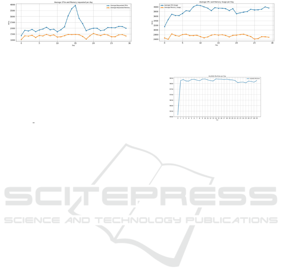
The result is plotted in Figure 5a. The immediate ob-

servation is that the average CPU request spikes and

reaches its maximum value on day 15. This is inter-

esting, as day 15 is also the day with the minimum

job activity in the whole trace period. This could in-

dicate that the job count for that day is so low that

the jobs submitted had tasks that were expected to be

CPU intensive, causing the allowed number of jobs to

be submitted to drop.

4.3.2 Resource Usage

We ﬁrst determine the average CPU and memory con-

sumption by tasks per day to perform the comparison.

The way these values are calculated is analogous to

that of the average resource request, the exception be-

ing that instead of summing the total amount of re-

quests per trace window, we use the sum of all the

Figure 6: Available machines per day.

average task consumptions recorded in each window.

The average value for each day is then given as the

average of the 288 usage sums on that day. These av-

erage values are shown in Figure 5b for both CPU and

memory values. Contrary to the resource requests,

the average CPU usage does not reach its maximum

value on day 15. We expect this abnormality is due

to the exception values described previously, where

a request value is set to 0, which implies it is not

set a limit to the resources it may use on some ma-

chines. These values would lead to a higher consump-

tion on some days instead of the average requests,

which would be lowered.

4.4 Overall Cluster Usage

We perform the overall cluster usage analysis by ex-

amining the MachineEvents table to see how many

machines are available to the cluster, the rate at which

they are added and removed, how many resources are

readily available to jobs and how much of those re-

sources are used. We assume the number will remain

relatively consistent throughout the trace. The result

can be seen in Figure 6, conﬁrming our prediction.

We can see that the cell we are analyzing has between

9800 and 9850 machines available every day through-

out the trace.

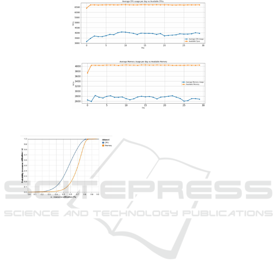
We also calculate the normalized sums of the

available CPU cores and RAM sizes that these ma-

chines provide, comparing with the resource usage

of tasks, showing us how much of these are actively

used. The comparisons are shown in Figure 7a and

Figure 7b. The units in these graphs are normalized

compute units (Wilkes, 2020a). The ﬁrst observa-

tion is that the available CPU and memory resources

stay consistent, despite the frequent additions and re-

CLOSER 2022 - 12th International Conference on Cloud Computing and Services Science

260

(a) Average CPU usage vs Availability per day.

(b) Average Memory usage vs Availability per day.

Figure 7: Average usage of resources vs their availability per day.

Figure 8: Cumulative graph displaying the probability of

the cell’s resource utilization being at most x.

movals of machines per day. Furthermore, as we

can see, the average resource consumption by tasks

never reaches the full capacity of the cell. The maxi-

mum average CPU usage occurs on day nine and uses

roughly 60% of the total capacity. For memory, the

maximum average usage takes place on day two of

the trace and consumes around 70% of the total ca-

pacity. Therefore, in general, this cell has around at

least 40% of its compute power lying idle daily and at

least around 30% of its memory capacity unused.

As an additional evaluation, we present a cumula-

tive graph of the probability of overall consumption

of CPU and memory resources in Figure 8. The x-

axis in this graph displays the percentage of the to-

tal resources utilized. The y-axis shows the proba-

bility of the utilization being at most x at any given

point in time during the trace. As we can observe, the

probabilities rise drastically as of around 40% total re-

source utilization, with the maximum probability be-

ing reached at around 80%. We gather from this, that

at no point in time during the trace was there more

than 80% of the total capacity of the cell being used.

4.5 Infrastructure Scalability

Evaluation

We have evaluated the scalability of the Dataproc-

based Infrastructure by determining the time taken by

the resource-usage calculation job on two different

types of machines cluster: machine1 with 4 vCPU

and 12GB memory, and machine2 with 2 vCPU and

6GB memory. Figure 9 shows the evaluation results

for the two types of machines with a different number

of worker nodes. It can be observed that the time re-

quired for characterizing the workload traces steadily

decreases with the number of worker nodes for both

types of machines. Additionally, the values become

almost constant as the worker nodes reach greater

than 12. Notably, machine2 with 4, 8, 12 and 16

worker nodes have almost the same completion time

as the machine1 at 2, 4, 6 and 8 worker nodes respec-

tively. For instance, around 280 seconds is observed

when worker nodes are above 8. This is attributed

to the fact that both clusters have approximately the

same number of cores and memory, leading to the

same performance.

5 CONCLUSION

Hosting workloads considering the heterogeneous na-

ture of cloud characteristics has been a pivotal point of

research for several cloud researchers and infrastruc-

ture providers in the recent past. A diligent charac-

terization of workloads eases infrastructure providers

and cloud developers. However, an efﬁcient charac-

terization approach of traces for the modern cloud

execution models such as serverless functions is not

Scalable Infrastructure for Workload Characterization of Cluster Traces

261

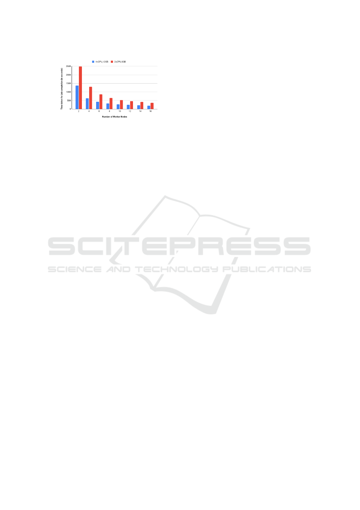
Figure 9: Dataproc-based infrastructure scalability evalua-

tion considering two types of virtual machines cluster hav-

ing different compute resources.

undertaken in the past. In this work, we studied the

Google cluster-traces v3 dataset, the latest of the

Google cluster traces, by analyzing its properties and

performing a workload characterization of the traces

using our proposed scalable infrastructure based on

Google Cloud Dataproc. We perform the workload

characterization on this dataset, focusing on the het-

erogeneity of the workload, the variations in job dura-

tions, aspects of resources consumption, and the over-

all availability of resources provided by the cluster.

Furthermore, we also show the scalability analysis of

the proposed infrastructure. The ﬁndings reported in

the paper will be beneﬁcial for cloud infrastructure

providers and users while managing the cloud com-

puting resources, especially serverless platforms.

In the future, we will further analyze missing in-

sights of the workload traces using our scalable in-

frastructure to study properties such as page cache

memory, CPI, and CPU usage percentiles to provide

further insights regarding the workload.

ACKNOWLEDGEMENTS

This work was supported by the funding of the Ger-

man Federal Ministry of Education and Research

(BMBF) in the scope of the Software Campus pro-

gram. Google Cloud credits in this work were pro-

vided by the Google Cloud Research Credits program

with the award number NH93G06K20KDXH9U.

REFERENCES

Alam, M., Shakil, K. A., and Sethi, S. (2015). Analysis and

clustering of workload in google cluster trace based

on resource usage.

Carreira, J., Fonseca, P., Tumanov, A., Zhang, A., and Katz,

R. (2019). Cirrus: A serverless framework for end-to-

end ml workﬂows. In Proceedings of the ACM Sym-

posium on Cloud Computing, pages 13–24.

Chadha, M., Jindal, A., and Gerndt, M. (2021).

Architecture-speciﬁc performance optimization of

compute-intensive faas functions. In 2021 IEEE

14th International Conference on Cloud Computing

(CLOUD), pages 478–483.

Cortez, E., Bonde, A., Muzio, A., Russinovich, M., Fon-

toura, M., and Bianchini, R. (2017). Resource central:

Understanding and predicting workloads for improved

resource management in large cloud platforms. In

Proceedings of the 26th Symposium on Operating Sys-

tems Principles, SOSP ’17, page 153167, New York,

NY, USA. Association for Computing Machinery.

Elgamal, T., Sandur, A., Nahrstedt, K., and Agha, G.

(2018). Costless: Optimizing cost of serverless com-

puting through function fusion and placement. CoRR,

abs/1811.09721.

Espe., L., Jindal., A., Podolskiy., V., and Gerndt., M.

(2020). Performance evaluation of container run-

times. In Proceedings of the 10th International Con-

ference on Cloud Computing and Services Science -

CLOSER,, pages 273–281. INSTICC, SciTePress.

Fan., C., Jindal., A., and Gerndt., M. (2020). Microservices

vs serverless: A performance comparison on a cloud-

native web application. In Proceedings of the 10th In-

ternational Conference on Cloud Computing and Ser-

vices Science - CLOSER,, pages 204–215. INSTICC,

SciTePress.

Gao, J., Wang, H., and Shen, H. (2020). Machine learn-

ing based workload prediction in cloud computing.

In 2020 29th International Conference on Computer

Communications and Networks (ICCCN), pages 1–9.

GoogleCloud (2016a). Bigquery documentation. Technical

report.

GoogleCloud (2016b). What is dataproc? Google cloud

documentation. Posted at https://cloud.google.com/

dataproc/docs/concepts/overview.

Guo, J., Chang, Z., Wang, S., Ding, H., Feng, Y., Mao, L.,

and Bao, Y. (2019). Who limits the resource efﬁciency

of my datacenter: An analysis of alibaba datacenter

traces. In Proceedings of the International Symposium

on Quality of Service, IWQoS ’19, New York, NY,

USA. Association for Computing Machinery.

Hellerstein, J. L. (2010). Google cluster data. Google re-

search blog. Posted at http://googleresearch.blogspot.

com/2010/01/google-cluster-data.html.

Kunde, S. and Mukherjee, T. (2015). Workload characteri-

zation model for optimal resource allocation in cloud

middleware. In 4th SAC 15: Proceedings of the 30th

Annual ACM Symposium on Applied Computing, page

442447.

Minet, P., Renault, r., Khouﬁ, I., and Boumerdassi, S.

(2018). Analyzing traces from a google data cen-

ter. In 2018 14th International Wireless Communica-

tions Mobile Computing Conference (IWCMC), pages

1167–1172.

Pacheco-Sanchez, S., Casale, G., Scotney, B., McClean, S.,

Parr, G., and Dawson, S. (2011). Markovian work-

load characterization for qos prediction in the cloud.

In 2011 IEEE 4th International Conference on Cloud

Computing, pages 147–154.

CLOSER 2022 - 12th International Conference on Cloud Computing and Services Science

262

Perennou, L., Callau-Zori, M., Lefebvre, S., and Chiky,

R. (2019). Workload characterization for a non-

hyperscale public cloud platform. In 2019 IEEE

12th International Conference on Cloud Computing

(CLOUD), pages 409–413.

Rasheduzzaman, M., Islam, M. A., Islam, T., Hossain, T.,

and Rahman, R. M. (2014). Task shape classiﬁcation

and workload characterization of google cluster trace.

In 2014 IEEE International Advance Computing Con-

ference (IACC), pages 893–898.

Reiss, C., Tumanov, A., Ganger, G. R., Katz, R. H., and

Kozuch, M. A. (2012). Heterogeneity and dynamicity

of clouds at scale: Google trace analysis. In Proceed-

ings of the Third ACM Symposium on Cloud Com-

puting, SoCC ’12, New York, NY, USA. Association

for Computing Machinery, Association for Comput-

ing Machinery.

Wilkes, J. (2011). More Google cluster data. Google re-

search blog. Posted at http://googleresearch.blogspot.

com/2011/11/more-google-cluster-data.html.

Wilkes, J. (2020a). Google cluster-usage traces v3. Tech-

nical report, Google Inc., Mountain View, CA, USA.

Posted at https://github.com/google/cluster-data/blob/

master/ClusterData2019.md.

Wilkes, J. (2020b). Yet more Google compute clus-

ter trace data. Google research blog. Posted at

https://ai.googleblog.com/2020/04/yet-more-google-

compute-cluster-trace.html.

Scalable Infrastructure for Workload Characterization of Cluster Traces

263