Total Cost Modeling for VNF based on Licenses and Resources

Ghoshana Bista

1,2

, Eddy Caron

1 a

and Anne-Lucie Vion

UMR CNRS - ENS Lyon, UCB Lyon 1 - Inria 5668, Lyon, France

Orange, Pessac, France

Keywords:

License Cost, Simultaneous Active Users, Software Licensing, VNF, Software Cost, Cloudiﬁcation, Soft-

warization.

Abstract:

Moving to NFV (Network Function Virtualization) and SDN (Software Deﬁned Network), Telco cloud archi-

tectures face four key challenges: interoperability, automation, reliability, and adaptability. All these chal-

lenges involve the optimization of resources; whether it is to increase the utilization of hardware resources

(virtualization) or to deliver shared computing resources and functions in real-time (cloudiﬁcation). Soft-

warization of networks is a consequence of telecom cloudiﬁcation. Virtual Network Function (VNF) is pro-

tected by IPR (Intellectual Property Right) like any software, ensured by a license describing usage rights and

restrictions at a given cost. Until now limited studies have happened in the economic dimension linked to

softwarisation. Currently, the telco industry struggles to converge and standardize licensing and cost models.

At risk: the network cloudiﬁcation beneﬁts could be swept away by poor management of resources (Hardware

and Software). This article presents a preliminary model for optimizing the total cost of a VNF, based on the

Resource Cost (RC) and License Cost (LC). This analysis is inspired by measurement and licensing practices

commonly observed in the Telcos industries,i.e consumption and capacity.

1 INTRODUCTION

NFV aims to increase automation and network reli-

ability for better and quicker service delivery. From

the research and markets, the global NFV market is

projected to grow from 12.9bn dollars in 2019 to

36.3bn dollars by 2024

. Also, 60 percent of ser-

vice providers will adopt NFV in the next two year

Service providers, more speciﬁcally telco companies,

need to adapt to this shift quickly and efﬁciently.

More than only technological challenges, historical

telcos must face the arrival of large hyper-scalers,

partners, and also aggressive competitors.

Service Providers will beneﬁt from NFV if they

can enable new services with a faster time-to-market,

rapidly scaling resources up and down, lowering the

costs. The key challenges facing NFV are thus linked

with resource optimization. Success relies on the abil-

ity to monitor and use standards and interoperable re-

sources: in other words, to mix and match various

software components on standard COTS (Commer-

cial -Off-The-Shelf) hardware.

https://orcid.org/0000-0001-6626-3071

https://www.f5.com/ f r

r/company/blog/why-nfv-is-

more-relevant-than-ever

As the network becomes software, failure in con-

trolling software spending destroys the promises of

NFV efﬁciency. The paradigm shift from equipment

property toward SW (Software) Right To Use (SW

RTU) is adding complexity in resource management.

As SW is protected by IPR over a license, it becomes

essential to ensure the compliance of SW deploy-

ments regarding acquired rights. As well, it becomes

essential to optimize license costs. For this, one of the

common practices in IT, extending to Network, is to

practice Software Asset Management (SAM). Imple-

menting end-to-end SAM guarantees that users buy

all the licenses user need, only the license need: to

avoid counterfeiting and waste.

SW license frames the rights and obligations of

the CSP (Communication Service Providers) to use

SW. License is associated with a cost (LC) which de-

pends on the volume of rights granted. The volume

granted and associated conditions of uses are contrac-

tually deﬁned by one or several metrics. There are

currently, no standards on metrics and their deﬁnition,

they depend on the creativity of software providers.

Which could facilitate every supplier of VNF to pro-

pose their metrics, model, and tools. And, this is be-

ing an intriguing and complex task for VNF services

246

Bista, G., Caron, E. and Vion, A.

Total Cost Modeling for VNF based on Licenses and Resources.

DOI: 10.5220/0011079600003200

In Proceedings of the 12th International Conference on Cloud Computing and Services Science (CLOSER 2022), pages 246-253

ISBN: 978-989-758-570-8; ISSN: 2184-5042

providers. Based on our observation on the telcos in-

dustries, metrics can be linked, among with usage, re-

source allocation, and resource consumption. Thus, it

is not wiser to consider LC and RC independently, but

we need to consider that LC can be dependent on the

resources and vice versa.

In this paper, we propose a model to evaluate and

optimize TCO (Total Cost of Ownership) of VNF de-

ployment based on LC and RC. We base our model

on two metrics; Simultaneous Active User (SAU) and

Bandwith (BW) as we observed that they are well

known in the telcos industries and can ﬁt both re-

source consumption, allocation, and capacity

textitOur contribution:

• We formulate the software cost model for VNF

based on LC, RC, and TC

• We introduce the concept of license reference,

which is crucial to anticipate the LC, RC, and TC.

• We provide different methods for licensing and

estimating its associated cost as LC, RC, and TC.

The rest of the paper is organized as follows: Sec-

tion 2 provides our related work and background.

Section 3 present our models and simulation and Sec-

tion 4 concludes this research.

2 BACKGROUND AND RELATED

WORK

2.1 Business Model

Our assumption of the business model is similar to

(Ahvar et al., 2017), which is deﬁned as (i) Service

provider, (ii) Network operator, (iii) VNF provider,

and (iv) User, customer or client, end-user. For us, a

service provider (SP) is a telco company that provides

communication services, network operator provides

servers, and operates infrastructure. VNF provider

is those that provide VNF and end-user are service

users. Different entities have different roles but these

can be changed or they can be operated by the same

entities too. Total Cost (TC) is calculated based on

LC (License Cost) and Resource cost (RC). Although

resources cost occasionally includes LC and various

other costs such as link, maintenance, upgrade, hard-

ware cost. In this study, we considered only RC

as VNF instances required to operate the necessary

amount of license (license reference). License is an

agreement that comes with rights and duties. The

right is to use a certain amount of SAU or BW in the

respective VNF and duties are to comply.

2.2 Related Work

Some researches were focused on optimizing the net-

work cost and the network path most of them include

LC as a constant entity. In (Mouaci et al., 2020) they

have dealt with ﬁnding the best place of VNF for a

better routing path for each demand this article helps

our research for ﬁnding the placement of SFC (Ser-

vice Function Chain). (Ahvar et al., 2017) had a sig-

niﬁcant impact on licensing but still, the authors did

not focus on the licensing cost or providing better op-

tions for clients. In (Kiran et al., 2020) they developed

VNFPRA problem which ﬁnds the optimal placement

of VNFs in SDN/NFV-enabled MEC (Mobile Edge

Computing) nodes to reduce the deployment and re-

source cost using genetic and mixed-integer prob-

lems. From this article, we get an idea about resource

allocation. In (Liu et al., 2019) they focused on the

placement of the VNF and trafﬁc steering using net-

work cost, node cost, and VNF placement cost. How-

ever, this article did not discussed the total cost and

optimizing LC but has illustrated a good insight into

in-network cost. In (Pham et al., 2017), Chuan Pham

et al. formulated problems for joint optimization and

trafﬁc cost optimization using the Markov Approxi-

mation (MA) in which they added their matching ap-

proach called SAMA. This research helps us to get

a proper idea of VNF instances, Although this work

was huge and concrete, they have not considered li-

cense cost or overall total cost. In (Shi et al., 2015)

authors focused on resources allocation of NFV com-

ponents using Markov Decision Process and Bayesian

learning which helped to dynamically allocate NFV

components.

3 FROM SYSTEM MODEL TO

SIMULATION

3.1 System Model

In this section, we provided cost models based on

VNF and traditional ways.

3.1.1 Traditional Ways

The popular traditional model is a perpetual license

and pay as you grow.

• Perpetual license: In this system users have to pay

upfront then only users have the right to use the

software. Depending upon the license entitlement

user can upgrade and update their software. Since

it is one-time pay generally it is highly expensive.

Total Cost Modeling for VNF based on Licenses and Resources

247

The dimension parameters used for a perpetual li-

cense are:

– LC

prl

: One time cost, upfront payment for li-

cense.

– RC

prl

: One time cost , upfront payment for re-

sources.

– TC

prl

: Total cost for perpetual license.

prl

= LC

prl

+ RC

prl

(1)

• Pay as you grow (PAYG): It is the model in which

end-user have to pay according to their capacity

increment, it can be usages based on resources,

services, or others. There are lots of pay-as-you

methods such as pay as you use, pay as you eat,

pay as you go, but for us, it is paid as you grow,

and grow here is in terms of SAU/BW. The dimen-

sion parameters used for the PAYG license model

are:

– no

= Number of SAU at a time.

– CS

PAY G

: Unit cost per SAU for license.

– CSr

PAY G

: Unit cost per SAU for resources.

– LCs

PAY G

: License cost for SAU.

– RCs

PAY G

: Resource cost for SAU.

– TCs

PAY G

: Total cost for SAU using PAYG.

LCs

PAY G

= Cs

PAY G

× no

RCs

PAY GS

= CSr

PAY G

× no

(2)

TCs

AY G = LCs

PAY G

+ RCs

PAY G

(3)

Now for the BW, dimension parameters are;

– no

: number of SAU at a time.

– CB

PAY G

: Unit cost per BW for license.

– CBr

PAY G

: Unit cost per BW for resources.

– LCB

PAY G

: License cost for BW.

– RCB

PAY G

: Resource cost for BW.

– TCB

PAY G

: Total cost for BW using PAYG.

LCB

PAY G

= CB

PAY G

× no

RCB

PAY GS

= CSr

PAY G

× no

(4)

TCB

PAY G

= LCB

PAY G

+ RCB

PAY G

(5)

One of the important points here not to forget is

that these are actually business models, not actual li-

censing models, they are only used as license mod-

els due to lack of the standard license models and

metrics. To ﬁll this gap we proposed license models

which ultimately help to construct optimized business

models in a virtual environment, VNF.

3.1.2 Virtual Network Function

Our crucial problem was to ﬁnd reliable and authentic

methods for licensing which would ultimately help to

model optimize the total cost in VNF. To address this

task we used the two important license metrics that

are SAU and BW (Bandwidth).

• SAU: SAU generally means simultaneous active

users connected with VNF who are consuming

some resources, and using services provided by

VNF.

• BW: It is related to the amount of bandwidth-

consuming/consumed by SAU.

• License reference: it is considered to be the es-

timated number of licenses required for the VNF

system for a certain period.

We choose these metrics among the other existing

metrics such as Transmission Per Second (TPS), Re-

quest Per Second (RPS), etc. because these metrics

are convenient to measure the usages and scalable pa-

rameters. Using these two metrics we created two

license reference (LR) models LR

(Equation (6))

and LR

(Equation (7)) respectively for SAU and

bandwidth, they can be formulated as follows;

= max

∀ j∈D



∑

∀i∈V

average(SAU

, j)



(6)

Similarly using BW,

= max

∀ j∈D



∑

∀i∈V

average(BW

, j)



(7)

where, V = (1, 2,.....v) is a set of all concerned

VNF (can be same or different type) in node. We de-

ﬁne H as a set of hours (1, 2, 3, ..., h), D as a set of

days (1, 2, 3, ..., d) and R as a set of License Refer-

ence (LR). LR corresponds to LR

or LR

which

we get from the Equations (6) and (7). Table 1 de-

lineates the parameters use in our formulation. Our

assumption for this research was that all VNFs were

deployed properly in their respective places and they

were functioning accurately in full capacity. These li-

cense references helped to generate an optimized total

cost model which includes license and resource cost

calculated as;

TC = RC

+ LC

(8)

Now, LC and RC can be calculated for capacity

model for a day, j ∈ D and r ∈ R, as:

= φ

+ σ

, (9)

= θ

+ δ

(10)

CLOSER 2022 - 12th International Conference on Cloud Computing and Services Science

248

LC and RC can be calculated for consumption

model for a day, j ∈ D, as:

= γ

× α

, (11)

= γ

× β

, (12)

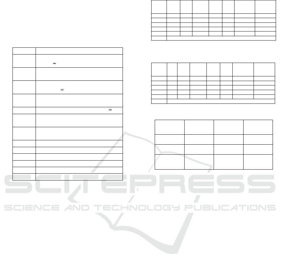
Table 1: Parameters use in problem formation.

r A License Reference. r ∈ R,

Pre-paid amount for License Refer-

ence (C),

Surpass or exceed License Refer-

ence r,

Unit cost of license for License Ref-

erence r (C/SAU or Mbps),

License factor for License Refer-

ence r,

θ Prepaid amount for resources (C),

Resources factor for License Refer-

ence r,

Unit cost of resources for License

Reference r,

License Reference for a day, j ∈ D,

License cost for capacity,

Resources cost for capacity,

License cost for consumption,

Resources cost for consumption.

D As a set of days (1, 2, 3, ..., d)

Now, implementing these equations (6), (7) and

(8) in different scenario, such as i) VNF instances sce-

nario ii) Users dependent iii) Using ﬂavour in nodes.

These scenarios are depends on users, usages, and

nodes.

3.2 Simulations

In this section, we deal with two types of use case

scenarios and a real scenario.

3.2.1 Scenario 1: VNF Instances

In this scenario, we presented different available

clients’ usages like; Web, VoIP, and Online Game.

We modiﬁed the table of (Pham et al., 2017) to ad-

just it to our model. For this scenario, users need to

be aware of their requirements based on SAU or BW.

Using SAU and BW the ﬂavour base table is proposed

on Table 2 and Table 3 which is supposed to meet the

user’s requirement. Importantly, license cost and re-

source cost mentioned in our tables are LC

and RC

i.e. license capacity and resources capacity cost.

So, if the trafﬁc requirement is BW (65Mbps) for

web services from Table 4 then for this services sim-

ulator proposed ﬂavour E and for VoIP simulator pro-

posed ﬂavour D. Whenever exact trafﬁc range require-

ment is not available simulator proposed higher value

Table 2: BW Flavour Table for Scenario 1 (VNF instances).

Flavour BW

(Mbps)

cost

(Ke)

vStorage

(TB)

vRAM vCPU Redundancy Resources

cost (Ke)

A 15 200 2 2 GB 2 1 170

B 20 250 3 2 GB 3 2 200

C 30 355 4 3 GB 4 2 285

D 50 435 4 3 GB 4 2 338

E 65 549 5 4 GB 4 2 420

F Customize your needs

Table 3: SAU Flavour Table for Scenario 1 (VNF in-

stances).

Flavour SAU LC

cost

(Ke)

vStorage

(TB)

vRAM vCPU Redundancy Resources

cost (Ke)

A 100 250 4 2 GB 2 1 100

B 150 350 4 3 GB 3 2 150

C 200 450 6 4 GB 4 2 215

D 250 550 7 5 GB 5 2 275

E 350 650 8 5 GB 5 2 325

F Customize your needs

Table 4: Service chain of different client usages with BW.

Client usage Service Chain Minimum

Trafﬁc Re-

quired (BW)

Minimum

Trafﬁc Re-

quired (SAU)

Web Services NAT-FW-

WOC-IDPS

65Mbps 165

VoIP NAT-FW-

TM-FW-NAT

35Mbps 200

Online Game NAT-FW-

VOC-WOC-

IDPS

150Mbps 300

NAT: Network Address Translator, FW: Firewall, TM: Trafﬁc Moni-

tor, WOC: WAN Optimization Controller, IDPS: Intrusion Detection

Prevention System, VOC: Video Optimization Controller

ﬂavour, and for the last online game since users re-

quirement is higher than the available option so users

either can be satisﬁed with ﬂavour D or the best op-

tion would be to customize their requirements with

services provider, i.e. ﬂavour E. So, in these kinds

of situation simulator directly proposed ﬂavour E. A

similar phenomenon goes for SAU as well. For web

services usage, ﬂavour C was proposed from Table 3.

Similarly, for VoIP, ﬂavour C matched the require-

ment too and for the online game, ﬂavour E covered

the user’s requirement. So using these ﬂavours based

tables the end-user can estimate the optimized total

cost.

3.2.2 Scenario 2: Users

The second scenario depends on the user. In this

research users were categorized in two types, Ê

Resources Know Users and Ë Resources Unknown

Users.

Ê Resources Known Users (RKU): These are the

users who know the estimated amount of resources

in terms of SAU/BW required for their system. In

this scenario, ﬂavour table was created based on SAU,

BW like in previous Table 2 and Table 3, also in

these tables total cost was introduced so that depend-

Total Cost Modeling for VNF based on Licenses and Resources

249

ing upon the user’s budget they can choose ﬂavours

too.

For this evaluation, a simulator had been cre-

ated named ﬂavour selector where users can input the

range of SAU, BW, and total cost depending upon

their requirement our simulator will propose the ap-

proximate ﬂavor. For example, if the SAU range

given by the client is 100-120 our selector suggests

ﬂavor A from Table 5. Another case is a range be-

tween 130-160 then our selector suggests ﬂavour B

also whenever the user inputs range value then it will

suggest customizing ﬂavor, i.e. ﬂavour E. Similar to

BW, if the client provides the range of bandwidth be-

tween 18-20 Mbps the selector will propose ﬂavour B

from Table 6. Another interesting case is using to-

tal cost. For the total cost, we added the value of

Resources Cost (RC

) and License Cost (LC

) as

shown in column (9

) in Table 5 and Table 6. So,

depending upon the customer’s budget simulator pro-

posed ﬂavour between SAU and BW. For example:

if the client’s budget range is from 800-900ke, the

simulator provides ﬂavour D from Table 5. Further-

more, if the range is from 600-700ke then it could be

from ﬂavour C from SAU or BW table. So, to avoid

the confusion of choosing between SAU and BW the

simulator asks the client preference between SAU and

BW. Thus, depending upon the client’s needs simula-

tor provides the result either from BW, SAU or cost.

Ë Resources Unknown Users (RUU): These are

the users who don’t have the estimated knowledge

about resources requirements (SAU, BW) for their

system. So for these types of users, a simulator was

created to provide the users with several choices. At

ﬁrst, users need to provide their range after which the

simulator will propose the least SAU value from the

Table 5. If the user is not satisﬁed with that proposed

then they can processed further simulator will pro-

pose from BW Table 6, least range from BW. If this

range is also not satisfactory to the client requirement

then the simulator proposed the mean value from the

SAU ﬂavour table, if this also fails to meet the user’s

needs the simulator proposed the mean value from

the BW ﬂavour table. After this, the simulator pro-

posed the highest value of SAU and BW from SAU

and BW ﬂavour table respectively. So the simulator

proposed from least to maximum ﬂavour value from

tables based on SAU, BW. Thus, our aim here is to

provide as many options as possible to the user. Ad-

ditionally, the offer can be made concerning the total

cost as performed in RKU.

3.2.3 Scenario 3: Node Analysis in Real Scenario

For this analysis, we used the two techno-economic

friendly models to estimate the LC, RC. They are

Table 5: SAU Flavour Table for Scenario 2.

Flavour SAU LC

(Ke)

vStorage

(TB)

vRAM vCPU Redundancy Resources

cost

(Ke)

Total

cost

(Ke)

A 100 250 4 2 GB 2 1 100 350

B 150 350 4 3 GB 3 2 150 500

C 200 450 6 4 GB 4 2 215 665

D 250 550 7 5 GB 5 2 275 825

E 350 650 8 5 GB 5 2 325 975

F Customize your needs

Table 6: BW Flavour Table for Scenario 2.

Flavour BW

(Mbps)

(Ke)

vStorage

(TB)

vRAM vCPU Redundancy Resources

cost (K

Total

cost

(Ke)

A 15 200 2 2 GB 2 1 170 370

B 20 250 3 2 GB 3 2 200 450

C 30 355 4 3 GB 4 2 285 640

D 50 435 4 3 GB 4 2 338 773

E 65 549 5 4 GB 4 2 420 969

F Customize your needs

capacity and consumption. To adapt these models

from a business point of view we have considered

some thresholds, constraints related to license and re-

sources like license threshold, resources threshold, li-

cense factors, etc.

• Capacity: The capacity analysis is similar to pre-

paid service where a certain amount of cost is

paid upfront to a certain capacity (license refer-

ence for our research) of VNF. When it surpasses

the threshold extra costs will be incurred. The

threshold can be a license or resource or both.

In this research both LC and RC were estimated

using unit cost and license reference using Equa-

tions (9) and (11). In this mode, once the capacity

is increased it cannot be reversed even if the con-

sumption (SAU/BW) is lower than the threshold.

• Consumption: Clients will pay for the resources

they had consumed or will consume during a cer-

tain time. As a consequence, there is no contrac-

tual threshold limiting the user’s ability to con-

sume resources (SAU, BW). It was calculated us-

ing Equations (11) and (12).

• LC threshold: This is the threshold for calculating

license cost. LC threshold was implemented for

both LC

and LC

. In this research, wherever li-

cense is being used it includes both (LC

, LC

It is deﬁned at the time of negotiation of the con-

tract based on estimated needs. If the uses exceed

the threshold, the cost of a license is increased by

1.5, 2, 3, . . . , n, which is known as license factor

σ. The license threshold is based on LR.

• RC threshold: It is the threshold in the resources.

Whenever a threshold is exceeded, it requires a

careful evaluation to understand whether the ex-

ceeded threshold can be covered by a single re-

source or more. If it can be covered with one re-

source then our research will use resources fac-

tor (δ)=1, and if requires more than one it will be

from 1,5, 2, 3, 4, 5, . . . , n. This threshold is also

dependent upon the LR. Alike the LC threshold, it

CLOSER 2022 - 12th International Conference on Cloud Computing and Services Science

250

can be negotiable between the VNF provider and

the SP.

• LC factor (σ): It is a multiplicative factor after ex-

ceeding threshold, σ= 1.5, 2, . . . , n. License factor

and resources factor were introduced here to cre-

ate a proper business model because whenever the

threshold is exceeded in the capacity model, the

service provider will charge some extra amount.

• RC factor (δ): It is similar to the LC factor but it

is in the resources aspect. δ= 1.5, 2, 3, . . . , n.

So, now using all these metrics and equations

(12) and (11) the total cost in consumption model be-

comes:

max

∀ j∈D

∑

(α

+ β

) (13)

Similarly, from equations (10) and (9) total cost

for capacity model became:

max

∀ j∈D

∑

(φ

+ σ

+ θ

+ δ

) (14)

A presumption was made that it will meet the QoS

threshold, T H

, i.e min TC ≤ T H

. T H

is not a nu-

merical value but a condition.

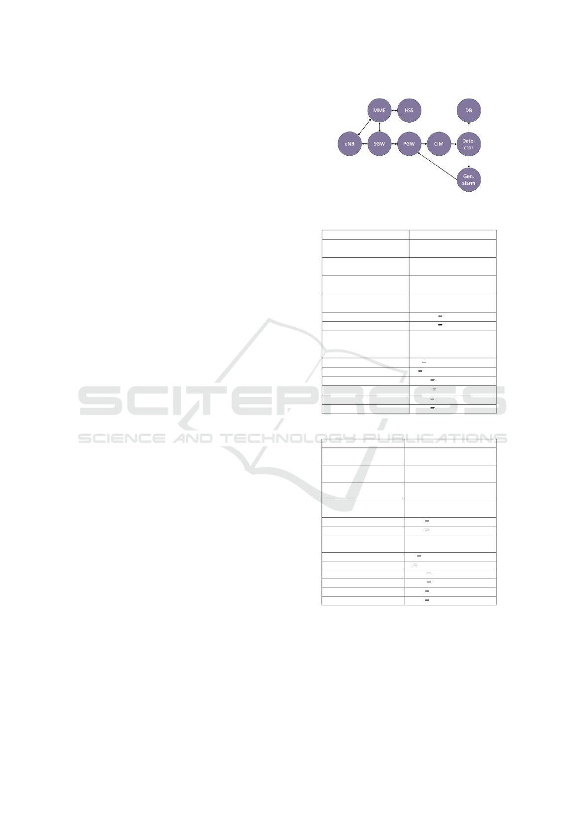
Now, for this situation, we considered a similar

scenario as in (Malandrino et al., 2019) i.e ICA (In-

tersection Collision Avoidance). ICA issues the alert

signal if any pair of them are about to collision. All

the parameters which were adapted to replicate the

business models are given in Table 7 and Table 8.

This simulation is executed on the Intel(R) Core(TM)

i7-6600U CPU @ 2.60GHz 2.81 GHz, 16GB RAM,

Windows 10. For the sake of simplicity, we as-

sume that resources can be scaled easily. We gen-

erated SAU and BW randomly on each virtual node,

also known as Virtual Evolve Packets (vEPC) such as

MME, SGW, PGW, etc. After the SAU and BW were

generated in each vEPC we implemented our license

reference model as in Equations (6) and (7) and ob-

tain the Figures 2 and 6 for SAU and BW. After the

estimation of license reference, we estimated the li-

cense cost using the Equations (9) and (11) and its

result is shown in the Figures 3 and 7. After success-

fully evaluating the LC we analyze the RC using the

Equations (10) and (12) with the help of the license

reference as shown in Figures 4 and 8. Further, we

estimated the total cost using Equations (13) and (14)

which were shown in Figures 5 and 9. The experiment

is carried out three times with three different random

values for thirty days and its cumulative average re-

sults are presented in all ﬁgures.

3.2.4 Evaluation

Figures 2 and 6 show the estimated license reference

based on randomly generated BW. Randomly gener-

Figure 1: VNF graph of the ICA service.

Table 7: Simulation parameter for SAU.

Parameters Value

License threshold for ca-

pacity

4725

Resource threshold for

capacity

4725

σ for both capacity for

1.5 (for LR less then

4725, 2 for LR >4725

δ 1.5 for SAU < 4725 and

2 for LR > 4725

θ 33000 (C)

φ 40000 (C)

SAU 500 add random(0,50),

random(0,100) and ran-

dom(10,1000)

α for SAU 10C per LR for License

β for SAU 6C per LR for Resource

PAY G

0.01(C) per SAU

CSr

PAY G

0.04 (C) per SAU

prl

500 (C)

prl

800 (C)

Table 8: Simulation parameter for BW.

Parameters Value

License threshold for ca-

pacity

Resource threshold for

capacity

σ for both capacity for

1.5 (for LR less then 65, 2

for LR >65)

δ 1.5 for SAU < 70 and 2 for

LR > 70

θ 700 (C)

φ 600 (C)

BW random(5,10),random(10,20)

and random(30,40)

α for BW 10 C per LR

β for BW 6 C per Resource

PAY G

0.01 (C) per BW

CBr

PAY G

0.04 (C) per BW

prl

500 (C)

prl

800 (C)

ated BW is also shown in the ﬁgures with help of

which pay as you grow and perpetual license and its

related cost were estimated. We can see on both ﬁg-

ures that daily BW is higher than the reference. It is

due to licensing reference being based on hourly av-

erage, maximum over a day from all concerned VNF

from Equations (6) and (7). Not to be confused that

daily SAU and BW shown in ﬁgures are 24 hours con-

Total Cost Modeling for VNF based on Licenses and Resources

251

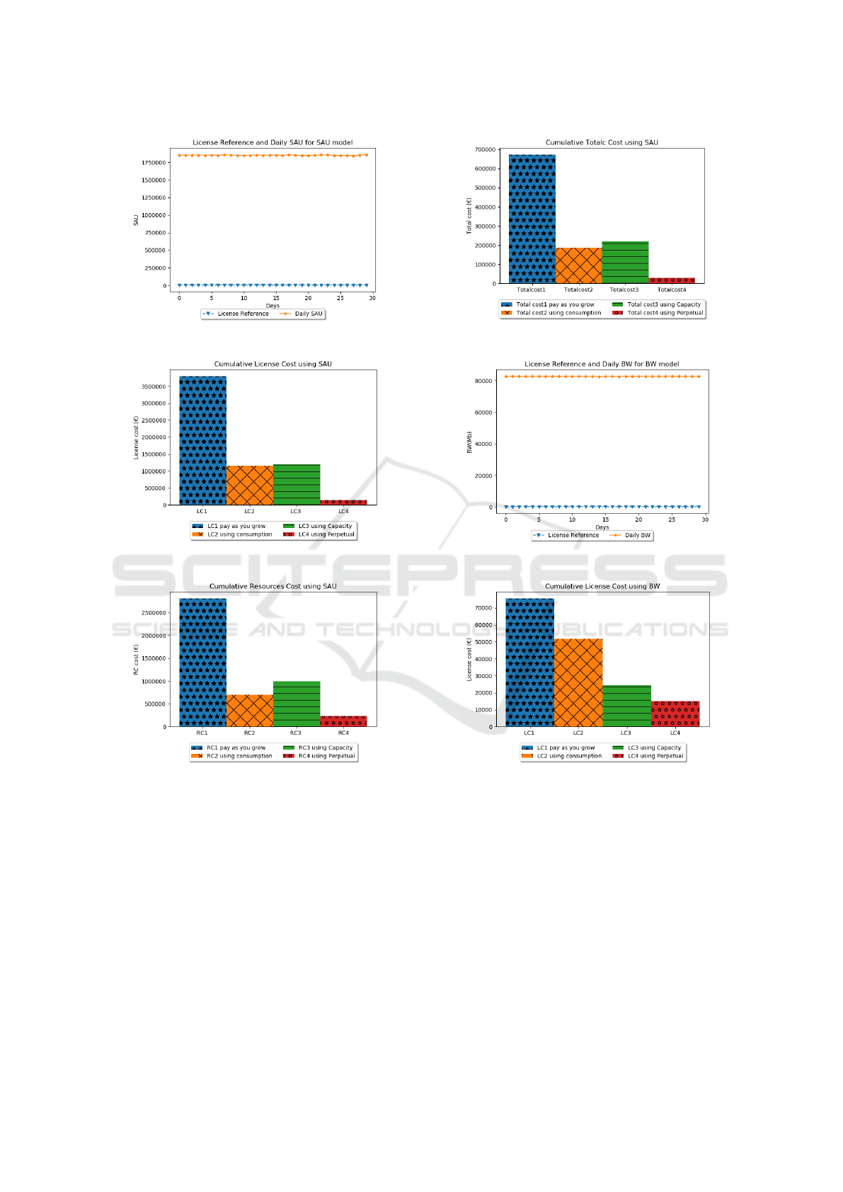
Figure 2: License Reference for SAU.

Figure 3: Cumulative License cost using SAU.

Figure 4: Cumulative Resource cost using SAU.

sumption by ICA service. Figures 3 and 7 which are

the cumulative license cost for 30 days we can see

that license cost using perpetual is lower and license

cost using pay as you grow is higher. An interesting

case here is license cost using consumption and ca-

pacity methods these are lower than pay as you grow,

among consumption and capacity, consumption has a

lower cost than capacity. One can argue that since

the perpetual cost is lower why not choose it but it

is not beneﬁciary for the VNF services provider. Be-

cause the perpetual model did not consider the usages

or resources consumption it is not fair for the VNF

services provider. Now, coming back to our ﬁgures in

Figure 5: Cumulative Total cost using SAU.

Figure 6: License Reference for BW.

Figure 7: Cumulative License cost using BW.

contrast with LC of SAU, BW LC for consumption is

higher and capacity is lower. Figures 4 and 8 show

that the consumption model estimated the lower re-

sources cost than the capacity in both SAU and BW.

Figures 5 and 9 show the estimated total cost. Fig-

ure 5 is the total cost for the SAU here we can see

that the consumption model estimated the lower cost

than capacity. While the BW capacity model esti-

mated the lower cost than consumption as shown in

Figure 9. One of the interesting points we can depict

from these ﬁgures is that when we use SAU as met-

rics with our models’ consumption model estimated

lower cost but in contrast of this when we use BW

CLOSER 2022 - 12th International Conference on Cloud Computing and Services Science

252

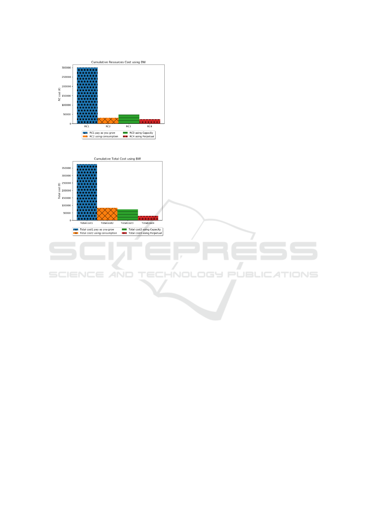
Figure 8: Cumulative Resource cost using BW.

Figure 9: Cumulative Total cost using BW.

as metrics with our models capacity model estimated

lower cost. This is due to the consumption of BW and

the number of SAU can not be compared, these are

two different metrics. SAU is a user connected with

the VNF and BW is the consumption of bandwidth

based on the SAU or services it consumes. This leads

us to the point that licensing could be done in differ-

ent ways depending upon the end-user requirement,

scenario, and QoS parameters (throughput, bit-rate,

etc). Also, different licensing metrics can be consid-

ered and depending upon the licensing metrics LC,

RC, and TC cost can be optimized. Thus, in simula-

tion for ICA when we use SAU as a metric consump-

tion model generated an optimized LC, RC and when

BW as a metric capacity model provided optimized

LC and RC.

4 CONCLUSIONS

The study has tried to suggest several models that are

relevant to the various scenarios. We compare the tra-

ditional ways of estimating total cost and our models

(capacity and consumption). Results conﬁrm that our

model is far better than the traditional one. We also

present different kinds of possible scenarios such as

VNF instances and Users which have a huge range of

requirements to be fulﬁlled. To meet the scenario re-

quirement, we proposed the ﬂavours methods (SAU,

BW). For users, we presented a solution based on to-

tal cost, SAU, and BW. Secondly, we implemented

our models in real VNF scenario ICA which clearly

shows that our models outperform other traditional

models it is because we introduced the concept of

license reference based on SAU and BW. So, from

all these, we can conclude that licensing is a com-

plex task that depends not only on one factor or met-

rics but also on several metrics, users, services, and

many others. We tried to include potential metrics

and constructed a novel model. Thus, we assume that

our models are not just limited to one scenario but

could be implemented on different circumstances and

topologies and will be helpful to estimate the opti-

mized total cost. Our future work will be to enhance

this model using DF, green energy, and implement it

on the more complex VNF SFCs.

REFERENCES

Ahvar, S., Phyu, H. P., Buddhacharya, S. M., Ahvar, E.,

Crespi, N., and Glitho, R. (2017). Ccvp: Cost-

efﬁcient centrality-based vnf placement and chaining

algorithm for network service provisioning. In 2017

IEEE Conference on Network Softwarization (Net-

Soft), pages 1–9. IEEE.

Kiran, N., Liu, X., Wang, S., and Yin, C. (2020). Vnf place-

ment and resource allocation in sdn/nfv-enabled mec

networks. In 2020 IEEE Wireless Communications

and Networking Conference Workshops (WCNCW),

pages 1–6. IEEE.

Liu, Y., Pei, J., Hong, P., and Li, D. (2019). Cost-efﬁcient

virtual network function placement and trafﬁc steer-

ing. In ICC 2019-2019 IEEE International Confer-

ence on Communications (ICC), pages 1–6. IEEE.

Malandrino, F., Chiasserini, C. F., Einziger, G., and Scalo-

sub, G. (2019). Reducing service deployment cost

through vnf sharing. IEEE/ACM Transactions on Net-

working, 27(6):2363–2376.

Mouaci, A., Gourdin,

E., Ljubi

C, I., and Perrot, N.

(2020). Virtual network functions placement and

routing problem: Path formulation. In 2020 IFIP

Networking Conference (Networking), pages 55–63.

IEEE.

Pham, C., Tran, N. H., Ren, S., Saad, W., and Hong, C. S.

(2017). Trafﬁc-aware and energy-efﬁcient vnf place-

ment for service chaining: Joint sampling and match-

ing approach. IEEE Transactions on Services Com-

puting, 13(1):172–185.

Shi, R., Zhang, J., Chu, W., Bao, Q., Jin, X., Gong, C., Zhu,

Q., Yu, C., and Rosenberg, S. (2015). Mdp and ma-

chine learning-based cost-optimization of dynamic re-

source allocation for network function virtualization.

In 2015 IEEE International Conference on Services

Computing, pages 65–73. IEEE.

Total Cost Modeling for VNF based on Licenses and Resources

253