Energy Demand Prediction in Hybrid Electrical Vehicles for Speed

Optimization

Daniel Fink

, Sean Shugar

, Zygimantas Ziaukas

, Christoph Schweers

, Ahmed Trabelsi

and Hans-Georg Jacob

Leibniz University Hannover, Institute of Mechatronic Systems, An der Universit

at 1, Garbsen, Germany

IAV GmbH, Berlin, Germany

Keywords:

Systems Modeling, Energy Demand Prediction.

Abstract:

Targeting a resource-efﬁcient automotive trafﬁc, modern driver assistance systems include speed optimization

algorithms to minimize the vehicle’s energy demand, based on predictive route data. Within these algorithms,

the required energy for upcoming operation points has to be determined. This paper presents a model-based

approach, to predict the energy demand of a parallel hybrid electrical vehicle, which is suitable to be used in

speed optimization algorithms. It relies on separate models for the individual power train components, and

is identiﬁed for a real test vehicle. On route sections of 5 to 7 km the averaged root mean square error for

the state of charge prediction results to 0.91 % while the required amount of fuel can be predicted with an

averaged root mean square error of 0.05 liters.

1 INTRODUCTION

A sustainable and resource-efﬁcient mobility is a key

challenge in reducing global warming. Intending to

meet this demand, the development of vehicles with

the lowest possible energy consumption is targeted

by manufacturers. Besides physical inﬂuences, such

as driving resistances, power train system and en-

gine characteristics, the vehicle’s energy demand de-

pends signiﬁcantly on the driver’s behavior (Radke,

2013). In this respect, increasing automation of the

vehicle control offers high potential to reduce the

energy demand. Therefore, considering the energy

demand within automated or assisted vehicle con-

trol algorithms is of particular importance to increase

the resource efﬁciency in automotive road transport

(Rosenzweig and Bartl, 2015).

Energy efﬁcient driving automation is part of current

research (H

ulsebusch, 2018). A common approach is

to plan and optimize a vehicle’s speed trajectory for

the upcoming route section. Usually, a dynamic pro-

gramming algorithm (Bellman, 2003) is used for the

the optimization process. In this process, an energy

model of a vehicle is called to determine the energy

requirements based on predictive route data. Within

such an optimization procedure, (Radke, 2013) uses

a prediction model for a combustion engine vehicle

to develop a driver assistance system for the vehi-

cle speed. Test drives indicate the fuel consump-

tion to be reduced by 10.2% when using this system.

(Freuer, 2016) demonstrates energy savings of up to

6% when optimizing the vehicle speed using an en-

ergy demand model for an electric vehicle. Applying

this approach within a risk-sensitive nonlinear model

predictive controller (Sajadi-Alamdari et al., 2020)

show that the energy efﬁciency of an electric vehicle

can be increased by 21%.

However, there is no investigation of other, more

complex drive concepts, such as parallel hybrid elec-

trical drives, to be used within a speed optimization

procedure described above. For these drives, litera-

ture provides many research works on energy man-

agement strategies (Zhang et al., 2020). Unfortu-

nately, these strategies are not suited to be applied

directly for any planning and optimizing approaches,

as they are usually based on adjusting the torque dis-

tribution. According to (H

ulsebusch, 2018), this ad-

justment is not possible in every assistant system. In

addition, the proposed strategies are mostly based on

vehicle simulations and are not veriﬁed under real

conditions. An approach that aims to predict the en-

ergy demand of hybrid electrical vehicles with a se-

ries drive conﬁguration is presented by (Fiori et al.,

2018). However, parallel drive conﬁgurations, which

are characterized by a complex torque distribution

mechanism, are not considered. Furthermore, (Pi-

116

Fink, D., Shugar, S., Ziaukas, Z., Schweers, C., Trabelsi, A. and Jacob, H.

Energy Demand Prediction in Hybrid Electrical Vehicles for Speed Optimization.

DOI: 10.5220/0011075600003191

In Proceedings of the 8th International Conference on Vehicle Technology and Intelligent Transport Systems (VEHITS 2022), pages 116-123

ISBN: 978-989-758-573-9; ISSN: 2184-495X

tanuwat et al., 2019) presents a hybrid vehicle energy

consumption model which only aims to determine the

consumed amount of fuel.

In this paper, we present a model based approach

to predict the energy demand of a hybrid electrical

vehicle with parallel working engines, based on route

data. This approach can be used within speed opti-

mization algorithms in driver assistance systems that

are not intended to be able to adjust the torque dis-

tribution. We build individual models for the single

power train components, such as combustion engine,

electric motor and battery as well as for the behav-

ior of the gearbox and the torque distribution control.

The model approaches are validated for a Volkswagen

Golf VII GTE using measured CAN data.

The paper is organized as follows. In section 2

we present the developed energy demand prediction

approach, introduce the separate models and demon-

strate the identiﬁcation process. In section 3 the pre-

sented approach is validated. Finally our results are

concluded in section 4.

2 ENERGY DEMAND MODELING

Algorithms to optimize a speed trajectory often rely

on dividing the global optimization problem into

smaller sub-problems. Usually, the solution space is

discretized and the optimal speed is determined only

for the transition between two discrete route points.

Previous vehicle states can not be taken into account.

Hence, it is required that the energy demand can be

determined only relying on the information of two

operation points. Therefore, the input values for an

energy demand model, which is suitable for common

speed optimization algorithms, are limited to distance

Δ 𝑑

𝑘

between two discrete operating points, as well

as to the velocities 𝑣

𝑘

, 𝑣

𝑘−1

and the route data based

heights ℎ

𝑘

, ℎ

𝑘−1

at both points.

2.1 Model Structure

Using a longitudinal vehicle model, as described in

(Mitschke and Wallentowitz, 2004), the required drive

wheel torque 𝑇

w,𝑘

to transit from operation point 𝑘 −

1 to operation point 𝑘 can be calculated for a given

dynamic rolling radius 𝑟

as follows:

𝑇

w,𝑘

(𝛼

𝑘

, 𝑎

𝑘

, 𝑣

𝑘

) = 𝑟

·(𝐹

a,𝑘

+𝐹

r,𝑘

+𝐹

g,𝑘

+𝐹

i,𝑘

). (1)

The road slope 𝛼

𝑘

and the occurring acceleration 𝑎

𝑘

are derived from the input information, by:

𝛼

𝑘

= arctan

ℎ

𝑘

−ℎ

𝑘−1

Δ 𝑑

𝑘

, (2)

𝑎

𝑘

(𝑣

𝑘

−𝑣

𝑘−1

)

+2 ·𝑣

𝑘−1

·(𝑣

𝑘

−𝑣

𝑘−1

)

2 ·Δ 𝑑

𝑘

. (3)

Furthermore, 𝑣

𝑘

represents the average speed within

the transition between the operation points. The driv-

ing resistance forces, such as the aerodynamic drag

force 𝐹

a,𝑘

, the gradient force 𝐹

g,𝑘

, the rolling resis-

tance force 𝐹

r,𝑘

and the inertia force 𝐹

i,𝑘

can be de-

termined, based on the deﬁned input information and

known vehicle parameters, as follows:

𝐹

a,𝑘

𝜌 ·𝑐

· 𝐴

·𝑣

𝑘

, (4)

𝐹

g,𝑘

= 𝑚

·𝑔 ·sin 𝛼

𝑘

, (5)

𝐹

r,𝑘

= 𝑐

·𝑚

·𝑔 ·cos 𝛼

𝑘

, (6)

𝐹

i,𝑘

= 𝑚

·𝑒

·𝑎

𝑘

. (7)

Here, 𝜌 is the density of air, 𝑐

the aerodynamic drag

coefﬁcient, 𝐴

the vehicle frontal area, 𝑔 the gravita-

tional acceleration, 𝑚

the vehicle mass, 𝑐

the rolling

resistance coefﬁcient, and 𝑒

an additional factor to

consider rotational masses.

In parallel hybrid electrical power trains, the

torque, applied by the two individual engines, cannot

be derived from the required wheel torque directly.

This torque additionally relies on the behavior of two

preconnected components. First, the gearbox which

Torque requirements

Transmission

Torque distribution

CEEM

Battery

Energy demand

𝑇

w,𝑘

𝑖

t,𝑘

𝑇

CM,𝑘

𝑇

EM,𝑘

𝐼

EM,𝑘

𝑈

EM,𝑘

𝑠

c,𝑘

¯𝑣

𝑘

𝑣

𝑘

, 𝑣

𝑘−1

Δ 𝑑

𝑘

ℎ

𝑘

, ℎ

𝑘−1

𝑇

Br,𝑘

𝑠

c,𝑘−1

Figure 1: Structure of the prediction approach.

Energy Demand Prediction in Hybrid Electrical Vehicles for Speed Optimization

117

determines the transmission ratio between wheel axle

and output shaft of the engines. Second, the torque

distribution control which determines the part of to-

tal drive torque the single engines are required to ap-

ply. The behavior of these components depend on var-

ious unpredictable factors, such as the engine temper-

ature. Due to the limited input information within a

speed optimization procedure, these components can-

not be modeled in detail. However, their behavior

must be taken into account when predicting the partic-

ular torque and thus the energy demand of the individ-

ual drives. For this reason, we present an estimation

approach for both, transmission ratio and torque dis-

tribution before modeling the electric motor and the

combustion engine. The structure of our overall ap-

proach to predict the energy demand is demonstrated

in ﬁgure 1.

2.1.1 Transmission Estimation

The gear selection within the gearbox mainly depends

on the drive shaft speed and the torque to be transmit-

ted. As the these values are unknown at this stage

of the energy demand model (see ﬁgure 1), we aim

to estimate a transmission factor 𝑖

t,𝑘

based on vehicle

speed 𝑣

𝑘

and wheel torque 𝑇

w,𝑘

. Therefore, accord-

ing to (Nelles, 2001), we declare 𝑖

t,𝑘

for an operation

point 𝑘 to be a linear combination of weighted basis

functions, as follows:

𝑖

t,𝑘

(𝑇

w,𝑘

, 𝑣

𝑘

) =

𝑀

𝑖=1

𝑁

𝑗=1

𝑤

t,𝑖, 𝑗

𝑖

(𝑇

w,𝑘

, 𝜉

𝑖

)Φ

𝑗

(𝑣

𝑘

, 𝜂

𝑗

). (8)

A basis function Φ

𝑞

(𝑢, 𝒄) for the input 𝑢 and a set

of grid points 𝒄 is deﬁned to be a linear function that

equals 1 at a grid point 𝑐

𝑞

while it is 0 at the neighbor-

ing 𝑐

𝑞−1

and 𝑐

𝑞+1

and all other grid points, as declared

by:

𝑞

(𝑢, 𝒄) =











𝑢−𝑐

𝑖−1

𝑐

𝑖

−𝑐

𝑖−1

, if 𝑐

𝑖−1

≤ 𝑢 ≤ 𝑐

𝑖

𝑢−𝑐

𝑖+1

𝑐

𝑖

−𝑐

𝑖+1

, if 𝑐

𝑖

< 𝑢 ≤ 𝑐

𝑖+1

0, otherwise.

(9)

In order to determine the weights 𝑤

t,𝑖, 𝑗

in equation

(8) and thus, to identify the transmission behavior of

our test vehicle, we deﬁne 𝑀

= 23 grid points 𝜉

𝑖

for

the drive wheel torque 𝑇

and 𝑁

= 21 grid points 𝜂

𝑗

for the vehicle speed 𝑣.

We measure standard CAN data of the test vehi-

cle in drive sequences of 5 to 7km and create a data

set of 525 km in total which consists of 𝐿 = 293, 512

measured operating points for the drive shaft speed

𝑛

∗

, the vehicle speed 𝑣

∗

, the total power train torque

𝑇

∗

, the electric motor torque 𝑇

∗

, the electric motor

current 𝐼

∗

, the electric motor voltage 𝑈

∗

, the bat-

tery current 𝐼

∗

, the battery voltage 𝑈

∗

and the bat-

tery’s state of charge (SOC) 𝑠

∗

. Based on this data,

the drive wheel torque can be calculated using equa-

tion (1) and the actual transmission factor 𝑖

∗

t,𝑘

for a

single data point 𝑘 can be approximated by

𝑖

∗

t,𝑘

𝑛

∗

d,𝑘

𝑛

w,𝑘

2 ·𝜋 ·𝑟

·𝑛

∗

d,𝑘

60 ·𝑣

∗

𝑘

. (10)

Taking this transmission factor for given data points, a

least square algorithm, as described in (Nelles, 2001),

is used to determine a optimal set of weights 𝒘

t,opt

𝒘

t,opt

= argmin

𝒘

𝐿

𝑘=1

(𝑖

t,𝑘

−𝑖

∗

t,𝑘

)

, (11)

for an identiﬁcation data set containing about 83% of

the driving sequences in the data set.

2.1.2 Torque Distribution

Using the estimated transmission factor, the required

total drive or breaking torque 𝑇

can be derived from

the wheel torque. The total drive torque is applied

either by a single or by a combination of two power

train components such as electric motor, combustion

engine and braking system. In order to estimate how

the different components are addressed, we introduce

a torque distribution estimation approach. We deﬁne

this estimation to cover all procedures of distributing

the required drive torque to the individual drives.

The components to be addressed differ for the

states driving or decelerating. In driving state, the re-

quired torque is applied through the electric motor,

the combustion engine or by a combination of both.

In case of decelerating or braking the required torque

is a combination of the electric motor’s recuperative

torque and a braking torque at the wheels. For this

reason, we consider the states driving and decelerat-

ing separately.

Decelerating State. As the recuperating ability is

limited, the required torque can be applied only to a

certain extend by the electric motor when decelerat-

ing. The remaining part of the required deceleration

torque must be applied through the braking system. In

order to model this behavior, the method described in

section 2.1.1 is used. At deceleration states the elec-

tric motor’s recuperative torque 𝑇

EM,𝑘

(𝑇

t,𝑘

, 𝑠

c,𝑘

) is as-

sumed to rely on the total required torque 𝑇

t,𝑘

, as well

as on the battery’s SOC 𝑠

c,𝑘

𝑇

EM,𝑘

(𝑇

t,𝑘

, 𝑠

c,𝑘

) =

𝑀

𝑖=1

𝑁

𝑗=1

𝑤

EM,𝑖, 𝑗

𝑖

(𝑇

t,𝑘

, 𝜉

𝑖

)Φ

𝑗

(𝑠

c,𝑘

, 𝜂

𝑗

) (12)

VEHITS 2022 - 8th International Conference on Vehicle Technology and Intelligent Transport Systems

118

We deﬁne 𝑀

= 7 grid points for the total torque and

𝑁

= 7 grid points for the SOC to determine a set of

weight for the recuperation torque estimation at de-

celeration stages. We use the identiﬁcation data set,

as described in section 2.1.1, to ﬁnd an optimal set

of weights according to equation (11). However, only

data points at deceleration states (𝑇

t,𝑘

< 0) are used

for the identiﬁcation. While the identiﬁcation data al-

ready contains a measured SOC value for every single

operating point, it is unknown at this stage of the pre-

diction approach. Compared to other vehicle states,

the SOC can be assumed to change signiﬁcantly less

dynamically. Therefore, the previous SOC 𝑠

c,𝑘−1

used for the recuperation torque estimation. As the

braking torque dissipates from the system, it is not

further considered for the energy demand prediction.

Driving State. At driving state, the torque distribu-

tion mainly depends on the required total drive torque

and the vehicle speed. In addition, we assume that the

total required drive torque is always fully distributed

between electric motor and combustion engine. This

allows to deﬁne 𝑟

𝑘

as a distribution ratio between

electric motor torque 𝑇

EM,𝑘

and combustion engine

torque 𝑇

CE,𝑘

by:

𝑟

𝑘

𝑇

CE,𝑘

𝑇

t,𝑘

𝑇

CE,𝑘

𝑇

CE,𝑘

+𝑇

EM,𝑘

. (13)

In order to determine the torque distribution behavior

at driving states, we declare

𝑟

𝑘

(𝑇

t,𝑘

, 𝑣

𝑘

) =

𝑀

𝑖=1

𝑁

𝑗=1

𝑤

r,𝑖, 𝑗

𝑖

(𝑇

t,𝑘

, 𝜉

𝑖

)Φ

𝑗

(𝑣

𝑘

, 𝜂

𝑗

), (14)

and deﬁne 𝑀

= 11 grid points for the total torque and

𝑁

= 8 grid points for the vehicle speed. We use the

identiﬁcation data set as described in section 2.1.1. As

the torque distribution is additionally affected by the

SOC, we determine separate optimal weight sets for

ﬁve different SOC-ranges.

2.2 Electric Power Train

Electric Motor. To model the energy demand of the

electric part of the power train, we derive the motor’s

mechanical power 𝑃

m,EM, 𝑘

from its torque 𝑇

EM,𝑘

and

rotational drive shaft speed 𝑛

d,𝑘

, according to (Binder,

2018), as follows:

𝑃

m,EM, 𝑘

= 2𝜋 ·𝑇

EM,𝑘

·𝑛

d,𝑘

, (15)

where 𝑛

d,𝑘

results from equation (10). In contrast to

the gearbox and the torque distribution, characteristic

diagrams are usually available for the vehicle’s drives.

The energy demand of the electric motor depends on

it’s electrical power 𝑃

el,EM, 𝑘

, which is represented by

the sum of mechanical power 𝑃

m,EM, 𝑘

and the power

loss 𝑃

l,𝑘

𝑃

el,EM, 𝑘

= 𝑃

m,EM, 𝑘

+𝑃

l,𝑘

. (16)

The power loss 𝑃

l,𝑘

can be obtained by the interpo-

lation of a characteristic diagram for given values of

the rotational drive shaft speed 𝑛

d,𝑘

, the motor torque

𝑇

EM,𝑘

and the voltage 𝑈

EM,𝑘

that is applied to the mo-

tor. In order to determine the motor voltage at this

stage of the prediction approach, we assume 𝑈

EM,𝑘

be a bi-quadratic function of the SOC 𝑠

c,𝑘−1

and the

motor torque 𝑇

EM,𝑘

as follows:

𝑈

EM,𝑘

(𝑠

c,𝑘−1

,𝑇

EM,𝑘

) = 𝑝

𝑈

+ 𝑝

𝑈

·𝑠

c,𝑘−1

+ 𝑝

𝑈

·𝑠

c,𝑘−1

+ 𝑝

𝑈

·𝑇

EM,𝑘

+ 𝑝

𝑈

·𝑇

EM,𝑘

(17)

Using a least square algorithm, we ﬁnd an error min-

imizing parameter set 𝒑

𝑈

based on measured mo-

tor voltage values within the identiﬁcation data, de-

scribed in section 2.1.1. Having an approximation of

the motor voltage, according to (Binder, 2018), the

motor current can be derived from the electrical power

as follows:

𝐼

EM,𝑘

𝑃

el,EM, 𝑘

√

3 ·𝑈

EM,𝑘

· 𝑝

𝐼

. (18)

As the power factor 𝑝

𝐼

(also known as cos 𝜙) is un-

known for the electrical motor of our test vehicle, it

is identiﬁed, using a least square algorithm based on

measured motor current values within the identiﬁca-

tion data described in section 2.1.1.

Battery. Finally, we model the battery of the elec-

tric power train. According to (Elgowainy, 2021) the

amount of energy 𝐸

B,𝑘

, that is extracted from or sup-

plied to the battery, can be determined by:

𝐸

B,𝑘

= 𝑈

B,𝑘

·𝐼

B,𝑘

·Δ 𝑡

𝑘

. (19)

While the time interval Δ 𝑡

𝑘

between two operation

points can be derived from the input values Δ 𝑑

𝑘

and

𝑣

𝑘

, the battery’s voltage 𝑈

B,𝑘

and its current 𝐼

B,𝑘

are unknown. However, the current at the battery

mainly depends on the motor current. We describe

this dependence by deﬁning a second order polyno-

mial function:

𝐼

B,𝑘

= 𝑝

𝐼

B,1

·𝐼

B,𝑘

+ 𝑝

𝐼

B,2

·𝐼

B,𝑘

+ 𝑝

𝐼

B,3

, (20)

in which an optimal parameter set 𝒑

𝐼

is to be found,

by using a least square algorithm, based on measured

battery current values within the identiﬁcation data

set, as described in section 2.1.1. Depending on the

battery current 𝐼

B,𝑘

and the motor voltage we deﬁne

the battery voltage 𝑈

B,𝑘

𝑈

B,𝑘

= 𝑈

EM,𝑘

+ 𝑝

𝑈

·𝐼

B,𝑘

, (21)

Energy Demand Prediction in Hybrid Electrical Vehicles for Speed Optimization

119

and ﬁnd the parameter 𝑝

𝑈

also by using a least

square algorithm, based on measured battery voltage

values within the identiﬁcation data set. To determine

the resulting SOC 𝑠

c,𝑘

, at the current operation point

𝑘, we relate 𝐸

B,𝑘

to the total effective energy content

of the battery 𝐸

t,eﬀ

and add it to the SOC of the pre-

vious operation point 𝑠

c,𝑘−1

as follows:

𝑠

c,𝑘

= 𝑠

c,𝑘−1

𝑈

B,𝑘

·𝐼

B,𝑘

·Δ 𝑡

𝑘

𝐸

t,eﬀ

. (22)

2.3 Combustion Engine

For a combustion engine the fuel rate

𝑄

g,𝑘

for an op-

eration point 𝑘 can usually be derived from a char-

acteristic diagram which is speciﬁed by the manufac-

turer. In order to derive the correlating energy demand

𝐸

CM,𝑘

from this consumption and thus to combine it

with the energy demand of the electric power train

part 𝐸

B,𝑘

, the heating value of gasoline 𝐻

is used as

follows:

𝐸

CM,𝑘

𝑄

g,𝑘

·Δ 𝑡

𝑘

·𝐻

, (23)

where Δ𝑡

𝑘

represents the past time between operation

point 𝑘 −1 and 𝑘.

3 VALIDATION RESULTS

Using the prediction approach presented in section 2

the energy demand of both engines can be determined

based on route data and velocity values. To validate

this approach, the data set described in section 2.1.1

is split into 6 parts. For an evaluation of the predic-

tion accuracy we perform a 6-fold cross validation, in

which 6 times 5 different data set parts are used for

the identiﬁcation procedure, while the remaining part

is preserved for validation.

The required elevation proﬁles for the validation

drive sequences are obtained by using a HERE rout-

ing API (HERE Maps, 2021) on the sequences’ GPS

values. Based on the measured vehicle speed 𝑣

∗

, and

the obtained elevation ℎ

∗

, the energy demand is deter-

mined separately for each validation drive sequence

using the presented approach. Thereby, only the ﬁrst

measured SOC value of a drive sequence is used,

while hereafter the prediction approach relies on SOC

values predicted in previous steps. Thus, the remain-

ing SOC measurements are only used for evaluation

purposes. In order to asses the prediction accuracy,

a root mean square error is determined between pre-

dicted and measured values. This error value is cal-

culated for each of the 6 different validation data sets

within the 6-fold cross validation procedure and than

averaged.

In addition, the prediction behavior of the single

power train component models is evaluated and visu-

alized on a data set independent test drive sequence, to

analyze the error propagation through the prediction

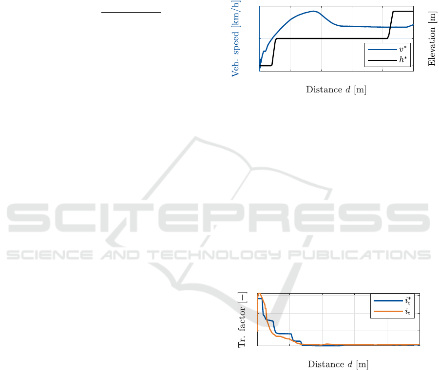
approach. For this purpose, ﬁgure 2 shows the vehicle

speed and the elevation proﬁle for the ﬁrst kilometer

of the test drive sequence.

0 200 400 600 800 1000

100

Figure 2: Vehicle speed and elevation proﬁle.

Based on this input data, the transmission factor is

predicted, as described in section 2.1.1, and compared

to the actual transmission factor, which is calculated

from the measured power train speed and the vehicle

speed, according to equation (10). While ﬁgure 3 il-

lustrates this comparison for the test drive sequence,

the averaged root mean square error results to 0.407

for the 6-fold cross validation on the entire data set.

The transmission factor’s value range of our test ve-

hicle extends from 2.44 for the sixth gear to 13.76 for

the ﬁrst gear. The predicted transmission factor values

𝑖

show a reasonable ﬁt for the test drive. However, the

gearbox-related staged transmission behavior, during

the dynamic acceleration stage, can only be predicted

approximately.

0 200 400 600 800 1000

Figure 3: Transmission factor prediction and measurement.

In order to illustrate the effect of the predicted

transmission factor, ﬁgure 4 shows the 𝑖

-based pre-

diction of the total power train torque 𝑇

, compared to

the actual measured value 𝑇

∗

. The comparison shows

that even in areas where the transmission factor is not

ﬁtting properly, such as between 100 m and 200m, the

total torque prediction proves an adequate behavior.

However, an occurring peak of high torque at 65m

is not met after a short interruption in the accelera-

tion procedure (see ﬁgure 2). The averaged root mean

square error on the validation data results to 27.19 Nm

in a value range for the total torque from −220 Nm to

VEHITS 2022 - 8th International Conference on Vehicle Technology and Intelligent Transport Systems

120

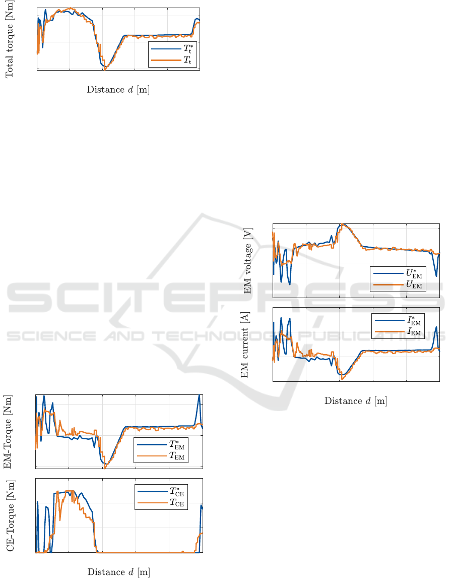
250Nm.

0 200 400 600 800 1000

-200

200

Figure 4: Total torque prediction and measurement.

The torque distribution, relying on 𝑇

, is evalu-

ated by comparing each engine’s torque, calculated

by using the predicted distribution ratio 𝑟 according

to equation (13), with measured engine torque values.

The 6-fold cross validation on the total data set leads

to an averaged root mean square error of 23.11Nm

for the electric motor torque and 17.33 Nm for the

combustion engine torque. Figure 5 shows the pre-

dicted combustion engine torque 𝑇

as well as the

predicted torque of the electric motor 𝑇

compared

to the measured values 𝑇

∗

and 𝑇

∗

for the test drive

sequence. Both predictions illustrate a reasonable ﬁt.

However, there are two areas to be pointed out. First,

the early peaks of the measured combustion engine

torque, at 20 m and at 70 m, are not met. Here, the

engine was switched on shorty, which could not be

predicted. This mismatch can be traced to the incor-

rect total torque determination in this areas (see ﬁgure

4). Second, in the area from 140 m to 180 m the torque

distribution is also inaccurate. It can be seen that the

torque is predicted to be applied by a combination of

both engines, while the measured values indicate that

the combustion engine drives the vehicle all by itself.

-200

200

0 200 400 600 800 1000

100

200

300

Figure 5: Prediction and measurement of engine torques.

The partly higher errors in predicting the torque

distributions are probably caused by the simpliﬁca-

tion of assuming that the procedure of distributing

the required drive torque is only depending on SOC

and vehicle speed. Actually, this task is performed

by a complex control algorithm that relies an many

additional internal power train states, such as engine

temperature. Furthermore, the distributing behavior is

not only depending on the current operation point, but

also on previous states. Thus, even if the current oper-

ation point indicates, that the torque can be applied by

the electric motor only, the combustion engine might

be still supporting. This can be due to higher torque

requests in previous operation points and a delayed

shutdown behavior. However, this and other inﬂu-

ences can not be considered in the torque distribution

model, as the purpose of the prediction approach is

to be applied within optimization algorithms. These

algorithms neither propagate previous states nor de-

tailed internal power train values.

340

360

380

0 200 400 600 800 1000

-100

100

200

Figure 6: Prediction and measurement of current and volt-

age at the electric motor.

Based on the electric motor torque, the prediction

of the electric motor’s current and voltage are eval-

uated. Figure 6 shows the predicted motor current

𝐼

and the voltage 𝑈

where the propagation of

the torque prediction errors are evidently reﬂected.

The voltage root mean square error results to 2.93 V,

in a value range of 320 V to 400 V. The root mean

square error for the motor current is determined as

16.83A, for occurring values between −100 A and

200A. However, these error dimensions are caused

by the preceding errors in predicting the motor torque

values. When validating the motor voltage and cur-

rent prediction based on measured torque values 𝑇

∗

the root mean square errors can be found as 1.74 A for

the motor current and 1.69V for the motor voltage.

Energy Demand Prediction in Hybrid Electrical Vehicles for Speed Optimization

121

-200

-100

100

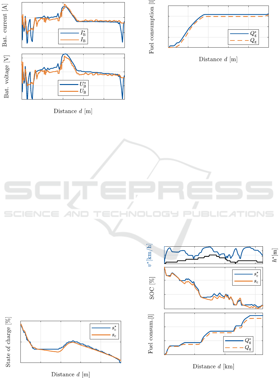
0 200 400 600 800 1000

360

370

380

Figure 7: Prediction and measurement of current and volt-

age at the battery.

A similar dependence on prediction errors for the

electric motor torque is indicated by the two predicted

battery states current 𝐼

and voltage 𝑈

in ﬁgure 7.

Here, a root mean square error of 16.75A is deter-

mined for the battery current while this value equals

2.7A when validating the prediction based on mea-

sured electric motor torque values 𝑇

∗

. For the bat-

tery voltage a root mean square error is found to equal

3.13V on a predicted electric motor torque and results

to 0.99V for measured torque values.

Finally, the prediction of the required SOC is eval-

uated. For this purpose, the SOC 𝑠

is determined,

based on previously predicted states of the electri-

cal power train, as described in section 2.2. Figure

8 shows the comparison of 𝑠

with measured values

𝑠

∗

for the selected test drive sequence. It is indicated

that the preceding inaccuracies, in particular for the

torque peaks mentioned above, are not affecting the

SOC prediction too much. The predicted values 𝑠

indicate a reasonable ﬁt. However, deviating torque

predictions, persisting over a longer distance, are re-

ﬂected in the SOC prediction, as the area between

200m and 400 m shows. Within the validation proce-

dure the root mean square error for the SOC predic-

tion is found to equal 0.91%. A validation of the SOC

0 200 400 600 800 1000

Figure 8: State of charge prediction and measurement.

0 200 400 600 800 1000

0.02

0.04

0.06

0.08

Figure 9: Prediction and measurement of the required

amount of fuel.

prediction, based on measured electric motor torque

values, leads to a root mean square error of 0.84 %.

Regarding the combustion engine part of the

power train, the prediction of the required amount of

fuel is validated. Figure 9 shows the comparison of

the predicted 𝑄

and the measured fuel consumption

𝑄

∗

for the test drive sequence. Here, the impact of

the not predicted combustion engine torque peaks at

20m and 70m (cf. ﬁgure 5) forms out. The measured

values increase sharply, due to the engine’s switch-

on process, which usually requires a relatively high

amount of fuel, compared to its normal operation.

This results in a remaining gap between the predicted

and the measured fuel consumption. The torque de-

viations in the areas 140 m to 180 m and 260 m to

350m are less effecting the consumption prediction,

as for the corresponding operating points the speciﬁc

fuel requirements do not differ as much. The valida-

tion procedure leads to a root mean square error of

0.05liters when relying on the predicted torque distri-

bution, while this error value equals 0.02 liters based

on combustion engine torque measurements.

100

0 2 4 6

0.1

0.2

Figure 10: SOC and fuel prediction for the entire test drive

sequence compared to measurements.

VEHITS 2022 - 8th International Conference on Vehicle Technology and Intelligent Transport Systems

122

In order to outline the behavior of the prediction

approach over a longer distance, ﬁgure 10 illustrates

the SOC and fuel consumption prediction for the en-

tire test drive sequence of 6.5 km.

4 CONCLUSION

In this paper, an approach is presented to predict the

energy demand of a hybrid electrical vehicle, based

on route data and speed values. The approach is build

to be suitable for an application within optimization

algorithms, as it only relies on input data for a single

transition between two operation points. The predic-

tion procedure is composted by a series of individual

models that represent the behavior of the single power

train components and can be described as follows.

For given speed and elevation values in two con-

secutive route points, the required drive torque at the

wheels is calculated using a longitudinal vehicle dy-

namic model. Further, a gearbox model is build and

identiﬁed to estimate the transmission behavior, based

on the wheel torque and vehicle speed. In order to de-

termine which part of the required total drive torque

will be applied by the individual drives, a model is

build to estimate a torque distribution ratio, based on

the total drive torque, the vehicle speed and the pre-

vious state of charge. Having the separate torque val-

ues, the combustion engine’s required amount of fuel

can be derived from a characteristic diagram. For the

electric part of the power train, the current and the

voltage are estimated and used within a battery model

to determine the required electric energy.

A data set of 525 driven kilometers is created to

identify and validate the prediction approach on a

Volkswagen Golf VII GTE. Using drive sequences of

5 to 7km within a 6-fold cross validation procedure,

an averaged root mean square error of 0.91 % can be

determined for the prediction of the state of charge.

Regarding the prediction of the amount of fuel re-

quired by the combustion engine, this error value re-

sults to 0.05 liter. The main part of prediction inaccu-

racies can be attributed to the estimation of the single

torques, to be applied by the individual engines. In

dynamic driving situation, in which both engines are

required, the estimation approach is not always capa-

ble to predict the correct distribution of the required

total drive torque. This might be approved by a more

complex model or by including the current accelera-

tion, when estimating the torque distribution. In ad-

dition, future work will investigate data-driven meth-

ods, such as neural networks, for their ability of esti-

mating the energy demand. Other advantages can be

assumed in involving more than one previous opera-

tion point, if they are given within the target applica-

tion of the prediction approach.

REFERENCES

Bellman, R. E. (2003). Dynamic programming. Dover Pub-

lications, Mineola, N.Y.

Binder, A. (2018). Elektrische Maschinen und Antriebe:

Grundlagen, Betriebsverhalten. Springer Berlin Hei-

delberg, Berlin, Heidelberg, 2. auﬂ. 2017 edition.

Elgowainy, A., editor (2021). Electric, Hybrid, and Fuel

Cell Vehicles. Springer eBook Collection. Springer

New York and Imprint Springer, New York, NY, 1st

ed. 2021 edition.

Fiori, C., Ahn, K., and Rakha, H. A. (2018). Micro-

scopic series plug-in hybrid electric vehicle energy

consumption model: Model development and valida-

tion. Transportation Research Part D: Transport and

Environment, 63:175–185.

Freuer, A. (2016). Ein Assistenzsystem f

ur die en-

ergetisch optimierte L

angsf

uhrung eines Elektro-

fahrzeugs. Springer Fachmedien Wiesbaden, Wies-

baden.

HERE Maps (2021). https://www.here.com/platform. (last

viewed 03/11/2022).

ulsebusch, D. (2018). Fahrerassistenzsysteme zur en-

ergieefﬁzienten L

angsregelung - Analyse und Opti-

mierung der Fahrsicherheit. PhD thesis, Karlsruher

Institut f

ur Technologie.

Mitschke, M. and Wallentowitz, H., editors (2004). Dy-

namik der Kraftfahrzeuge. VDI-Buch. Springer

Berlin Heidelberg, Berlin, Heidelberg and s.l., vierte,

neubearbeitete auﬂage edition.

Nelles, O. (2001). Nonlinear System Identiﬁcation: From

Classical Approaches to Neural Networks and Fuzzy

Models. Springer eBook Collection. Springer, Berlin

and Heidelberg.

Pitanuwat, S., Aoki, H., IIzuka, S., and Morikawa, T.

(2019). Development of hybrid vehicle energy con-

sumption model for transportation applications—part

ii: Traction force-speed based energy consumption

modeling. World Electric Vehicle Journal, 10(2):22.

Radke, T. (2013). Energieoptimale L

angsf

uhrung

von Kraftfahrzeugen durch Einsatz vorausschauen-

der Fahrstrategien. Karlsruher Schriftenreihe

Fahrzeugsystemtechnik. KIT Scientiﬁc Publishing.

Rosenzweig, J. and Bartl, M. (2015). A review and analysis

of literature on autonomous driving. The Making of

Innovation, pages 1–57.

Sajadi-Alamdari, S. A., Voos, H., and Darouach, M. (2020).

Ecological advanced driver assistance system for opti-

mal energy management in electric vehicles. IEEE In-

telligent Transportation Systems Magazine, pages 92–

109.

Zhang, F., Wang, L., Coskun, S., Pang, H., Cui, Y., and Xi,

J. (2020). Energy management strategies for hybrid

electric vehicles: Review, classiﬁcation, comparison,

and outlook. Energies, 13(13):3352.

Energy Demand Prediction in Hybrid Electrical Vehicles for Speed Optimization

123