Applying Edge AI towards Deep-learning-based Monocular Visual

Odometry Model for Mobile Robotics

Frederico Luiz Martins de Sousa

, Mateus Coelho Silva

and Ricardo Augusto Rabelo Oliveira

Computer Science Department, Federal University of Ouro Preto, Ouro Preto, 35400-000, Brazil

Keywords:

Edge AI, Mobile Robotics, Deep Learning, Monocular Visual Odometry.

Abstract:

Visual odometry is a relevant problem considering mobile robotics. While intelligent robots can provide map-

ping and location tasks with a multitude of sensors, it is interesting to evaluate the ability to create models using

less information to create similar information. While traditional approaches consider computer vision aspects

of proposing solutions, they lack the application of modern perspectives as edge computing and deep learn-

ing. This text assesses the problem of evaluating the usage of deep-learning-based visual odometry models in

mobile robotics. We expect mobile robots to have embedded computers with limited computing technologies,

so we approach this problem through the Edge AI perspective. Our results displayed an improvement of the

model considering previous results. Also, we proﬁle the performance of hardware candidates to perform this

task in mobile edge devices.

1 INTRODUCTION

There are several concepts around the functioning of

mobile robotics systems. Among these concepts, an

important issue to solve in every one of these systems

is odometry (Aqel et al., 2016). There are several

techniques used to provide this information, includ-

ing wheel odometry, laser odometry, Global Position-

ing System (GPS), Global Navigation Satellite Sys-

tem (GNSS), Inertial Navigation System (INS), Si-

multaneous Location and Mapping (SLAM), and Vi-

sual Odometry (VO).

While many of these methods rely on speciﬁc sen-

sors or sensor fusion, Visual Odometry’s minimal re-

quirement is the usage of images. Although tech-

niques in this ﬁeld can be improved using a com-

bination of cameras or sensors (Yousif et al., 2015),

some proposals research the extent of monocular vi-

sual odometry techniques (Forster et al., 2014), which

work based on a single camera image. Even if depth

perception sensors or LIDARs sometimes support this

activity, it is crucial to understand software limitations

when providing these services using only visual infor-

mation.

https://orcid.org/0000-0002-8522-6345

https://orcid.org/0000-0003-3717-1906

https://orcid.org/0000-0001-5167-1523

VO frequently uses traditional computer vision

matching (Aqel et al., 2016) to perform the desired

odometry task. Nonetheless, it is necessary to com-

pare these techniques with modern AI-based solu-

tions. The advance of AI in edge computing enforces

this possibility, requiring an experimental apparatus

(Lee et al., 2018).

Previously, we experimented with the possibility

of creating deep learning models to solve the monoc-

ular odometry issue (de Sousa et al., 2021b) using a

single camera as sensor. These experiments validated

the usage of deep learning to generate the required in-

formation.

An edge-computing-based environment is essen-

tial when global positioning is not available. Also,

creating edge-AI-based solutions helps produce sim-

pler robots that can navigate through an environment.

In this work, we further explore this perspective to-

wards edge AI. We employed the training of a deep

learning method, which was later tested on hardware

candidates regarding proﬁling issues.

Thus, the main objective of this work is:

• An evaluation of the usage of Edge AI to provide

monocular visual odometry in a mobile robotics

system.

The remainder of this text is organized as follows:

we used Section 2 to present the theoretical references

Martins de Sousa, F., Silva, M. and Oliveira, R.

Applying Edge AI towards Deep-learning-based Monocular Visual Odometry Model for Mobile Robotics.

DOI: 10.5220/0011071600003179

In Proceedings of the 24th International Conference on Enterprise Information Systems (ICEIS 2022) - Volume 1, pages 561-568

ISBN: 978-989-758-569-2; ISSN: 2184-4992

561

that guide this work. In Section 3, we present the re-

lated works found in the literature and how they differ

from what is presented here. Section 4 assesses the

setup used to perform experiments, the model train-

ing stage, and the proposed validation tests. Finally,

we present the results from the experiments in Sec-

tion 5, and discuss the conclusions from this work in

Section 6.

2 THEORETICAL REFERENCES

In this section, we discuss the main theoretical con-

tents related to this work. We present a review on vi-

sual odometry and mobile robotics. We also discuss

how other authors assess the monocular visual odom-

etry issue using AI. These are the main concepts in-

volved in the creation of this solution. To complete

the purpose of mobile robotics, the author state the

need to understand the surroundings of the mobile

robot and its objective, named mission.

2.1 Mobile Robotics

As the name suggests, mobile robotics is the study of

mobile robots. Jaulin (Jaulin, 2019) states that mo-

bile robots are autonomous mechanical systems capa-

ble of moving through the environment. These sys-

tems are composed of three main modules: sensors,

actuators, and intelligence. Computations in the in-

telligence module perform the coordination of sens-

ing and actuation.

Kunii et al. (Kunii et al., 2017) assess the main

operational aspects of autonomous mobile robots in

three different steps. Initially, the robot needs to ac-

quire information based on the surrounding environ-

ment. Then, it should plan a trajectory based on the

acquired data. Finally, the robot should move towards

its goal. This ﬁnal step is also referred to in the liter-

ature as the robot’s mission.

Sensing and intelligence are required for acquir-

ing information and understanding the environment.

Intelligence modules are also applied into the path

planning stage and in the conversion into an acting

plan for the actuators. These stages relate directly to

the modules cited in the previous paragraph.

2.2 Monocular Visual Odometry

(MVO)

As discussed in Section 1, odometry is a relevant is-

sue within the context of mobile robotics systems.

This issue is part of the environmental perception dis-

cussed in the previous subsection, related to mobile

robots’ sensing and intelligence modules.

One of the ways discussed for this approach is

monocular visual odometry (MVO), which uses a sin-

gle camera as a sensing unit. This method is useful

for robots that rely on a single camera as the sensor

for monitoring the surroundings (Hansen et al., 2011;

Benseddik et al., 2014). Traditional VO and MVO

techniques rely on point-matching methods to create

the understanding of positioning in an environment.

2.3 Visual Odometry and AI

More modern ways of understanding mobile comput-

ers must consider AI as part of the integrative process.

As much as traditional MVO methods rely entirely on

computer vision, there is also a need to understand

how various AI models should perform under edge

computing and AI combinations. For this matter, we

must also understand how VO, MVO, and AI are re-

lated.

Li et al. (Li et al., 2018) suggests the usage of deep

learning to estimate the depth and obtain the VO. For

this matter, they use stereo images to train an outdoor

MVO proposal. Although they present a viable tech-

nique, their work relies on technologies and images

that do not relate directly to the context of this work.

Also, their approach was not tested in mobile edge

devices.

Lui et al. (Liu et al., 2019) display a similar ap-

proach as the previous one, including the usage of the

same dataset to train and test their processes. In this

case, they propose the usage of a different deep learn-

ing technique to provide the same service as before.

This work also shares the same differences with the

proposed solution as the previous work.

These works and others in the literature display

that AI mainly was used to estimate VO in open-world

situations based on vehicular appliances. The litera-

ture lacks the discussion of its usage towards mobile

robotics. Also, the authors developed their models but

mainly did not test their performance in mobile edge

devices to consider their performance in mobile de-

vices.

The discussion presented in this paper adds both

on the possibility of generating the data to train mod-

els for a targeted environment, as well as discusses

the possibilities of the presented technique in mobile

edge computing contexts.

ICEIS 2022 - 24th International Conference on Enterprise Information Systems

562

3 RELATED WORKS

In the work introduced by Mur-Artal et al. (Mur-

Artal et al., 2015), they present a SLAM algorithm

called Orb-SLAM. This algorithm performs SLAM

with both monocular and stereo cameras. Orb-SLAM

is not an odometry algorithm. However, it uses dif-

ferences between pixels to estimate the robot’s posi-

tion within the navigation environment. These calcu-

lations become necessary due to the localization prob-

lem, which the SLAM algorithm solves.

In their approach, authors based on the binary de-

scriptor ORB, introduced by Rublee et al. (Rublee

et al., 2011). The ORB algorithm envisions to relate

pixels in two different images that describe the same

scene. The only difference between these images is

their position and orientation. The algorithm sets a

point in the ﬁrst image and tries to relocate this point

in the second image. This procedure can be helpful in

use cases where there is a need to estimate movement

between two images.

Thus, this process is used in Orb-SLAM to esti-

mate motion and consequently output a position and

orientation in the navigation environment. So Orb-

SLAM uses classical image processing techniques to

output a robot’s positional data within the navigation

environment. Since the Orb-SLAM algorithm also

uses monocular cameras to output positional data, we

compare their solution to ours, and this comparison

can be observed in Section 5.

4 METHODOLOGY

In the previous methodology described in (de Sousa

et al., 2021b), we developed and validated an odom-

etry neural network application. The application is

based on a ROS-based (Robot Operating System)

robot with a SLAM capability through a LIDAR laser.

The employed SLAM technique builds the neural

network dataset together with images are related to

the SLAM map coordinates. Therefore, this method-

ology enabled the neural network’s training step.

We employed the Euclidean distance metric to

validate the odometry’s neural network localization.

This metric calculates the distance between the pre-

dicted and ground truth coordinates. Thus, the greater

the distance, the larger the neural network’s error.

Then, based on this validation metric, we choose the

ResNet50 as the backbone of our network.

In this work, we present an evaluation of the previ-

ously introduced neural network. As our approach has

an edge-ai constraint, it must achieve a feasible per-

formance in embedded devices. The model’s feasibil-

ity to edge-ai depends on its inference time. The infer-

ence time consists of how long the computing device

takes to process a frame through the neural network

and output odometry data. We analyzed the hardware

consumption and inference time across different em-

bedded devices to evaluate the neural network.

4.1 Experimental Setup

In our experimental setup, used for model evaluation,

we use the embedded device in our main robot, which

corresponds to a Raspberry Pi 4. We also evaluate

the model in NVIDIA Jetson embedded devices. In

speciﬁc, we use the Jetson Nano and Jetson TX2 NX.

These small form factor embedded devices offer con-

siderable processing power with low power consump-

tion. This processing power is even more evident in

Jetson family boards due to their GPUs. GPUs play

a crucial role in neural network inferencing since the

most popular frameworks offer an accelerated inter-

face for these devices.

In our work, we employed the framework Tensor-

Flow in the 2.4 version for the training and inferenc-

ing process. Regarding the Raspberry Pi, we used

the TensorFlow CPU version. On the other hand, we

used the GPU version for Jetson boards since it sup-

ports CUDA, the GPU compute acceleration library

for NVIDIA hardware.

Regarding the platform’s embedded hardware, all

the devices are ARM-based. The Raspberry Pi 4 has

a 64-bit Quad-Core Cortex-A72 CPU with 1.5Ghz

of clock speed. The Jetson Nano also counts with a

Quad-Core Cortex CPU, but it is a lesser version, the

64-bit A57 with a clock speed of 1.43Ghz. The criti-

cal difference between Jetson Nano and Raspberry is

the GPU. Nano’s GPU is an NVIDIA Maxwell-based

architecture with 128 CUDA cores. The CUDA cores

enable using the CUDA GPU computation acceler-

ation toolkit by NVIDIA, which increases inference

speed.

At last, the Jetson TX2 NX consists of a more

powerful module. It counts with 2 CPUs, one is a 64-

bit Dual-Core NVIDIA Denver processing unit, and

the latter is a Quad-Core ARM Cortex-A57. Its GPU

is a Pascal-based architecture (more modern than

Maxwell), with 256 CUDA cores. Besides enabling

CUDA toolkit usage, CUDA cores are NVIDIA’s

graphic processing unit, and as higher the number of

cores, the higher is the expected performance. An-

other aspect to observe is that all embedded devices

count with 4GB of RAM, shared between CPU and

GPU.

Applying Edge AI towards Deep-learning-based Monocular Visual Odometry Model for Mobile Robotics

563

4.2 Model Description

As previously displayed in Sousa et al. (de Sousa

et al., 2021b), we validated that the ResNet backbone

converged to our dataset and obtained the best results.

Thus, we employ the same technique in this work.

The model uses a ResNet50 as the backbone for

the proposed model. Then, we ﬂatten the output to ob-

tain the latent vector and apply a 1024-neuron dense

layer to obtain the X and Y coordinates for the odom-

etry. We retrained the model to obtain better perfor-

mance when compared to the previous work.

4.3 Model Training

Based on the ﬁndings in our last work, we retrained

the previous neural network. We employed model re-

training to decrease the neural network mean error.

The previously trained model had 6203 images in the

training dataset, while in this retraining, it was in-

creased to 8029 images.

Another change related to the previous training

process is the input resolution. As we increased the

number of data for training, we decreased the model’s

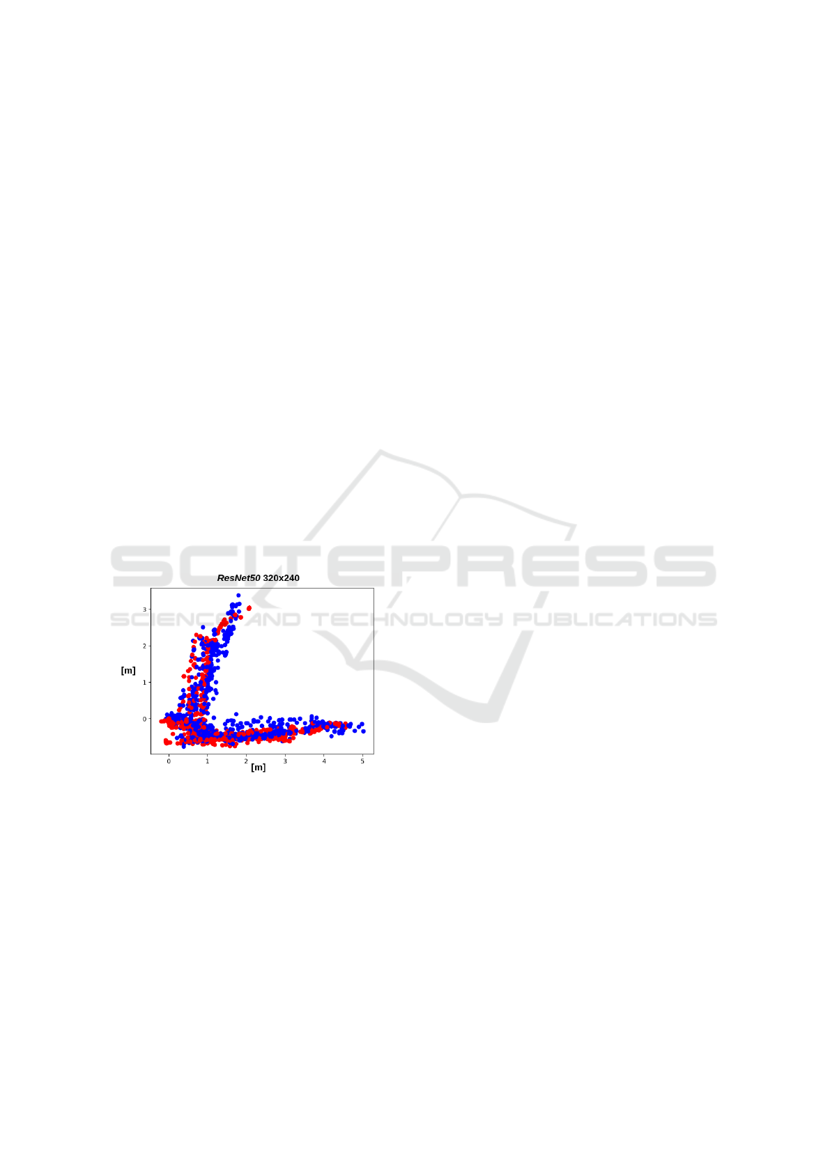
input resolution from 640x480 to 320x240. Figure 1

displays the comparison between the obtained results

and the ground truth.

Figure 1: Results obtained from the model training. The

red points display the ground truth, while the blue points

display the predicted values.

In Sousa et al. (de Sousa et al., 2021a), they show

that the model input resolution plays a crucial role in

edge performance regarding frames per second. This

resolution decrease aims at a better-embedded perfor-

mance in edge devices. We also changed the dataset

loading parameters. Through TensorFlow’s data input

interface, we employed a pixel normalization tech-

nique. This technique applies to all images within the

dataset where the mean pixel value is calculated. In

Section 5, we present the model’s mean error (based

on the Euclidean distance metric).

4.4 Validation Tests

After the model retraining process, we evaluated the

neural network’s hardware consumption and perfor-

mance in embedded devices. Thus, we used the FPS

(frames per second) as a metric for analysis for the

model’s performance evaluation. We calculate the

FPS based on the inference time of each embedded

platform. The FPS metric is helpful in use cases

where there is a need for real-time decisions. These

real-time constraints are deﬁned based on their ap-

plication, so all robot decisions must respect a pre-

deﬁned time.

We veriﬁed the memory, CPU, and GPU utiliza-

tion in each board regarding the hardware consump-

tion. This analysis is convenient for cases where mul-

tiple tasks need to execute in the same embedded de-

vice. The developed script for this analysis is quite

simple. It captures an image while the robot is tele-

operated in the navigation environment. Next, it con-

verts the image to the model’s input resolution then

sends the captured image for inferencing on the neu-

ral network through the TensorFlow interface. The

GPU consumption in this process is only measured in

the Jetson devices, as TensorFlow does not use GPU

in Raspberry’s case.

The second validation process of our approach

is based on a path comparison between our solution

and monocular Orb-SLAM. There are two versions of

Orb-SLAM, the monocular version (Mur-Artal et al.,

2015) and the stereo version (Mur-Artal and Tard

os,

2017). As we are working with visual odometry

through monocular cameras, we choose the monoc-

ular version of Orb-SLAM for comparison. However,

Orb-SLAM’s stereo version has a known better result

compared to its monocular counterpart.

Orb-SLAM is a SLAM algorithm and not an

odometry algorithm. However, we use the SLAM’s

localization technique to estimate the robot’s position

within the map and compare its projected trajectory.

This localization data outputted by the Orb-SLAM

algorithm generates the robot path. In Orb-SLAM’s

technique, they estimate the position through the def-

inition of points of interest on the frame. When these

points are deﬁned, the depth of each point is esti-

mated, then a 3D point cloud is created. These ﬁxed

points are used for distance and motion estimation be-

tween captured frames.

The algorithm calculates the robot’s position and

orientation within the navigation environment from

the previous techniques. One of the limitations of this

approach is the impossibility of a concrete displace-

ment estimation (in meters or centimeters) due to a

nonexistent known relation between the points (pix-

ICEIS 2022 - 24th International Conference on Enterprise Information Systems

564

els) deﬁned within the processed frame and the real

world. Therefore, the approach’s estimated positions

are all virtual estimations, which do not represent a

tangible measurement within the navigation environ-

ment.

The methodology of this test consists of creating

a route within the navigation environment and then

following it with the robot. The ﬁrst created route,

the ground truth route, uses the rf2o laser odometry

package (Jaimez et al., 2016). The outputs of this

odometry package are also used as ground truth for

the neural network. Then we compare this ground

truth between our odometry neural network predic-

tions and Orb-SLAM’s position outputs. The result

of this process can be observed in the next section.

5 RESULTS

In this section, we explore the results of the evaluation

process of our VO neural network. This evaluation

process consists of a previously introduced model re-

training evaluation. Then, we present a comparison

between the neural network’s predictions, a ground

truth, and Orb-SLAM positional data. Finally, we

introduce an embedded hardware consumption and

performance analysis based on three commonly used

edge devices.

5.1 Model Retraining Results

We compare the mean prediction error based on the

Euclidean distance to evaluate the model’s retraining

performance. This metric employs a calculation be-

tween a prediction and a ground truth position. The

previous model in our last work is a ResNet model

with an input resolution of 640x480. As described

in our methodology section, we retrained this model

with half of its resolution but with more data within

the training dataset. Table 1 shows the comparison

between these two models.

Table 1: Mean error comparison between previous and re-

trained models.

Model Mean Error (m) Std. Dev.

ResNet 640x480 0.4587 0.4924

ResNet 320x240 0.3519 0.3990

In Table 1 we can observe that the model’s retrain-

ing obtained a 23.28% decrease regarding the mean

error predictions. Despite the resolution decrease, the

mean error decreased at a considerable rate. How-

ever, this improvement is directly tied to the dataset

increase in sample number.

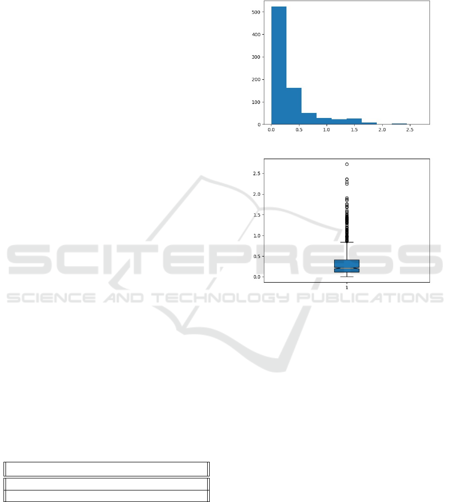
We also analyzed a histogram and a boxplot

of these errors to understand better how this error

spreads on the test dataset. Figure 2 and 3 present

the histogram and the boxplot respectively.

Figure 2: Retrained ResNet (320x240) error histogram.

Figure 3: Retrained ResNet (320x240) boxplot graph.

In blue, the interval where most value errors are spread

through the test dataset. The yellow line represent the pre-

diction error median. The black circles are the outliers.

The error histogram and the boxplot graph were

also evaluated in our last work. However, we observe

at least more than a hundred samples with a decreased

mean error. We also perceive that the number of out-

liers greater than 1.5 meters decreased. Also, regard-

ing the boxplot results, our maximum mean error is

below 1 meter, while the previous model was above

this value, around 1.3 meters.

5.2 Orb-SLAM Comparison

To compare and evaluate the VO neural network, we

compare its predictions with the ground truth. The

ground truth data was built with the laser odometry

package rf2o, which is the same package used to as-

semble the training ground truth. As mentioned in the

methodology section, we ﬁxed points on the ground

to the robot go through. In this process, we teleoper-

ated the robot following these ﬁxed points with each

strategy we compared. Figure 4 shows this compar-

Applying Edge AI towards Deep-learning-based Monocular Visual Odometry Model for Mobile Robotics

565

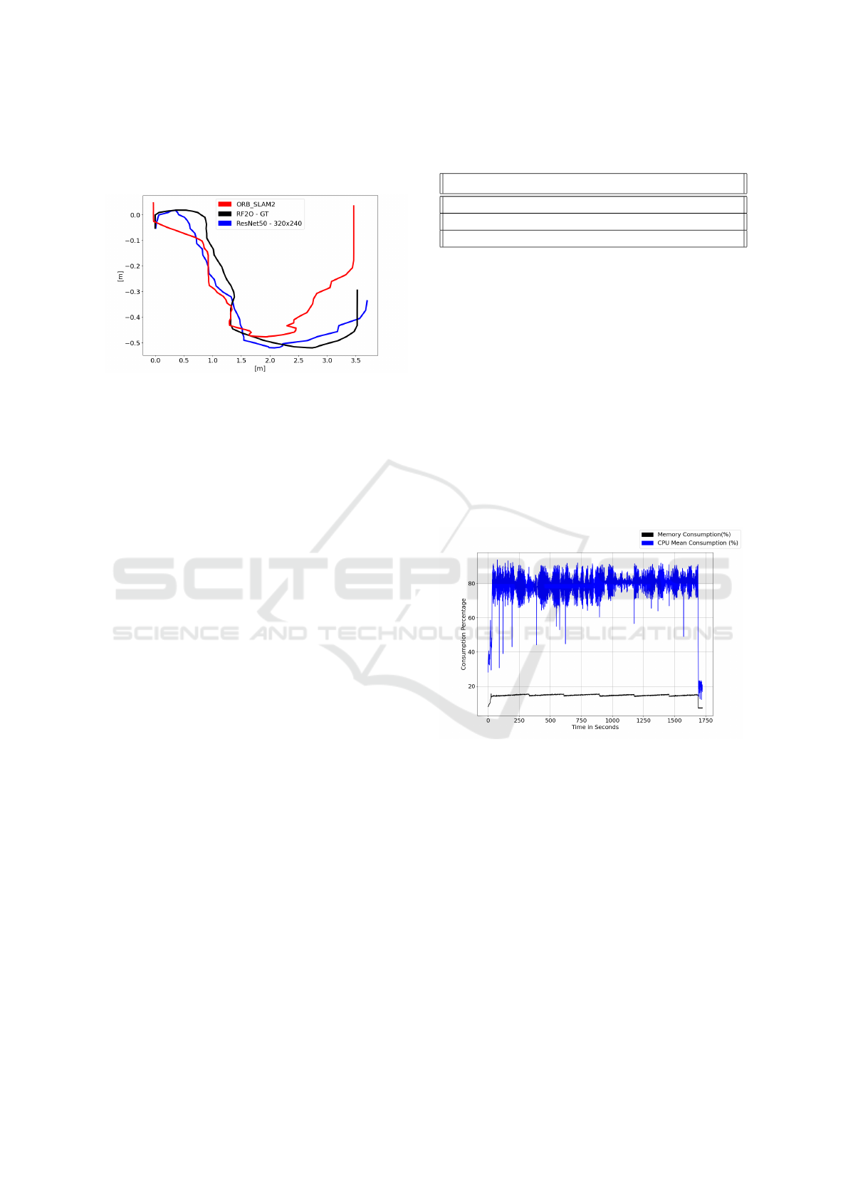
ison, in black the ground truth’s path, while in blue

there are our neural network predictions and in red

the Orb-SLAM positional data.

Figure 4: Path prediction comparison across the different

approached strategies. In black the ground truth predictions

based on the rf2o laser odometry. In blue the VO neural net-

work predictions. At last, in red the monocular Orb-SLAM

algorithm positional data.

As Figure 4 shows, our approach obtained a visu-

ally better output compared to the Orb-SLAM algo-

rithm. We also evaluated the paths with the Euclidean

distance metric. According to this metric, the path

predicted by the VO neural network had a mean error

of 25.47 centimeters compared to the ground truth’s

path. The error obtained is less than our mean er-

ror in the test dataset. The Orb-SLAM mean error

was 61.81 centimeters compared to the ground truth’s

route.

5.3 Hardware Consumption and

Performance Analysis

Our methodology section described the hardware de-

tails and frameworks for our tests. In this subsection,

we introduce a performance and hardware consump-

tion discussion. These are fundamental aspects as our

approach is an edge-ai application and needs deploy-

ment in embedded devices that rely on limited com-

putational resources.

The frames per second rate is a metric to evalu-

ate how fast the computer process each frame. This

metric is a deciding factor in a real-time application

where the robot needs to decide with a constraint of

time. In our approach, each image will output a posi-

tion (x, y) within the environment, and Table 2 shows

the mean inference time across all embedded devices.

As observed in Table 2, the higher framerate is

achieved by Jetson TX2 NX, as expected because

it has the best GPU. However, there is a noticeable

improvement in inference times when the GPU han-

dles the inference, which corresponds to Jetson’s case.

The performance improvement reaches a 95% rate in

Table 2: Performance comparison between the analyzed

edge devices.

Device Inference Time(s) FPS

Raspberry Pi 4 4.3 0.23

NVIDIA Jetson Nano 0.226 4.42

NVIDIA Jetson TX2 0.173 5.78

TX2 compared to the CPU inferencing on Raspberry.

It is worth mentioning that we disabled the Denver

CPUs in all tests carried on the TX2 board. The dis-

ablement was due to an issue described by the manu-

facturer, which, when these CPUs are enabled, delays

CUDA kernel latency. This delay affected our infer-

encing performance on this board, reaching a value

of 0.303 seconds for inferencing. This value increase

had an impact of 42.75% of inferencing time.

In Figure 5, we observe the mean CPU and RAM

consumption on the Raspberry when the inferencing

on the ResNet model is executed. The CPU consump-

tion ﬂoated between 70 to 85%. The memory con-

sumption sat around 20%. The memory usage peaks

at 540MB, while the idle system consumes 240MB,

representing a 125% increase.

Figure 5: Raspberry Pi hardware consumption in model in-

ferencing process. In blue there’s the mean CPU consump-

tion and in black the RAM consumption. The Y axis repre-

sent the use percentage and X axis represent the time.

In Figure 6, the Jetson Nano CPU, GPU, and

RAM consumptions are introduced. The mean CPU

load seats beneath 20%, while the memory usage

reaches a peak of 3GB, representing 75% of total sys-

tem memory. The idle system consumes only 400MB.

Finally, in Figure 7, the TX2 hardware consump-

tion is observed. The CPU consumption also settles

beneath a 20% load rate, while the memory usage

reaches an 80% rate. The idle memory consumption

is 500MB, and when the inferencing starts, the mem-

ory usage reaches a peak of 3.5GB.

Considering the presented hardware consumption

graphs, we consider that Raspberry CPU load for in-

ICEIS 2022 - 24th International Conference on Enterprise Information Systems

566

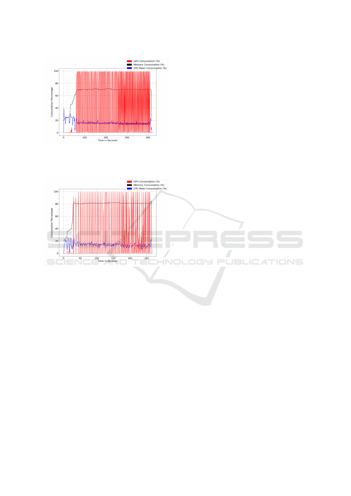
Figure 6: Jetson Nano hardware consumption in model in-

ferencing process. In blue there’s the mean CPU consump-

tion, in red the GPU, and in black the RAM consumption.

The Y axis represent the use percentage and X axis repre-

sent the time.

Figure 7: Jetson TX2 NX hardware consumption in model

inferencing process. In blue there’s the mean CPU con-

sumption, in red the GPU, and in black the RAM consump-

tion. The Y axis represent the use percentage and X axis

represent the time.

ferencing is not only slow (as Table 2 shows) but CPU

intense. Meanwhile, its memory consumption is con-

siderably decreased compared to Jetson boards. This

memory consumption difference can be due to the

neural network’s size and extra CUDA modules that

TensorFlow loads in Jetson devices to offer GPU ac-

celeration support. We also observe that the CPU is

less loaded in Jetson devices, which means that other

CPU applications can stage alongside the neural net-

work inference.

6 CONCLUSIONS

In this work, we introduced an evaluation of a neu-

ral network to solve a visual odometry problem. Our

approach is based on a previous paper in which we

validated a deep learning architecture for the visual

odometry problem. The methodology consisted of

testing the neural network in multiple scenarios where

we measured the hardware consumption and the per-

formance in embedded platforms. We also compared

our trained odometric neural network to a literature-

known algorithm called Orb-SLAM. The results ob-

tained by the tests indicate viability, mostly on Jet-

son boards. However, there is a need to evaluate a

real-time reference to properly analyze the neural net-

work’s viability related to the FPS result obtained in

edge devices.

In a ﬁrst model evaluation, the ResNet architec-

ture enabled a converge and better learn the naviga-

tion environment features. This model, in its retrained

version, obtained a mean error of 35.19 centimeters.

This value represents 7.68% of the maximal distance

in our navigation environment, which is 4.57 meters.

Compared to the last version of our model, the re-

training obtained more than 10 centimeters of error

decrease.

Secondly, we compared our neural network’s

solution with the known literature algorithm Orb-

SLAM. We evaluated the comparison through a

robot’s path differentiation in a graph. This graph

contained the path’s ground truth, the neural net-

work’s predictions, and the Orb-SLAM positional

outputs. We evaluated the obtained paths compared

to the ground truth using a Euclidean distance metric.

This process gave us a mean error of 25.47 centime-

ters compared to the ground truth and 61.81 centime-

ters in mean error to the Orb-SLAM compared to the

ground truth.

At last, we evaluated the hardware consumption

related to the frames per second across the described

embedded boards. The comparison was carried in the

following embedded platforms: Raspberry Pi 4, Jet-

son Nano e Jetson TX2 NX. We made the tests in

ARM Ubuntu operational system, with TensorFlow

on version 2.4. The tests showed that the best results

regarding the FPS were obtained on Jetson boards.

This result was expected due to the GPU accelera-

tion enabled by the CUDA toolkit support interface on

TensorFlow. Therefore, the CPU inferencing process

on Raspberry obtained a 0.23 FPS rate, Jetson Nano

achieved a 4.42 FPS rate, and ﬁnally, Jetson TX2 had

an FPS rate of 5.78 FPS.

Regarding the hardware consumption, in the

Raspberry Pi 4, the CPU consumption ﬂoated be-

tween 70 to 85% load. Meanwhile, its memory us-

age staged around 540 MB of consumption. In Jetson

boards, the GPUs are stressed to their limits, reach-

ing 100% load when there is a frame to be processed.

Despite the discrepancy in performance in favor of

the Jetson boards, we observed a high memory con-

Applying Edge AI towards Deep-learning-based Monocular Visual Odometry Model for Mobile Robotics

567

sumption in these devices. This increase in memory

consumption can be due to the extra CUDA mod-

ules loaded by TensorFlow to accelerate the infer-

encing process. At the same time, the memory us-

age increases at a rate of 548.15% on Jetson boards

compared to Raspberry, the performance tradeoff in-

creases at a rate of 2413% more performance regard-

ing the frames per second.

6.1 Future Works

In future improvements of this work, there is a need

to measure and evaluate the energetical consumption

of the embedded devices. Comparing energy-efﬁcient

edge-ai machines is crucial as most edge applications

rely on batteries. Energetical consumption is a con-

straint and critical aspect when inferencing neural net-

works at the edge. So to verify the actual applicability

of our neural network at the edge, it is interesting to

test the energy consumption for the completeness of

our work’s evaluation process.

ACKNOWLEDGEMENTS

The authors would like to thank FAPEMIG, CAPES,

CNPq, and the Federal University of Ouro Preto

for supporting this work. This work was partially

funded by CAPES (Finance Code 001) and CNPq

(308219/2020-1).

REFERENCES

Aqel, M. O., Marhaban, M. H., Saripan, M. I., and Ismail,

N. B. (2016). Review of visual odometry: types, ap-

proaches, challenges, and applications. SpringerPlus,

5(1):1–26.

Benseddik, H. E., Djekoune, O., and Belhocine, M. (2014).

Sift and surf performance evaluation for mobile robot-

monocular visual odometry. Journal of Image and

Graphics, 2(1):70–76.

de Sousa, F. L. M., da Silva, M. J., de Meira Santos, R.

C. C., Silva, M. C., and Oliveira, R. A. R. (2021a).

Deep-learning-based embedded adas system. In 2021

XI Brazilian Symposium on Computing Systems Engi-

neering (SBESC), pages 1–8. IEEE.

de Sousa, F. L. M., Meira, N. F. d. C., Oliveira, R. A. R.,

and Silva, M. C. (2021b). Deep-learning-based visual

odometry models for mobile robotics. In Anais Es-

tendidos do XI Simp

osio Brasileiro de Engenharia de

Sistemas Computacionais, pages 122–127. SBC.

Forster, C., Pizzoli, M., and Scaramuzza, D. (2014). Svo:

Fast semi-direct monocular visual odometry. In 2014

IEEE international conference on robotics and au-

tomation (ICRA), pages 15–22. IEEE.

Hansen, P., Alismail, H., Rander, P., and Browning, B.

(2011). Monocular visual odometry for robot localiza-

tion in lng pipes. In 2011 IEEE International Confer-

ence on Robotics and Automation, pages 3111–3116.

IEEE.

Jaimez, M., Monroy, J. G., and Gonzalez-Jimenez, J.

(2016). Planar odometry from a radial laser scan-

ner. a range ﬂow-based approach. In 2016 IEEE In-

ternational Conference on Robotics and Automation

(ICRA), pages 4479–4485. IEEE.

Jaulin, L. (2019). Mobile robotics. John Wiley & Sons.

Kunii, Y., Kovacs, G., and Hoshi, N. (2017). Mobile robot

navigation in natural environments using robust ob-

ject tracking. In 2017 IEEE 26th international sym-

posium on industrial electronics (ISIE), pages 1747–

1752. IEEE.

Lee, Y.-L., Tsung, P.-K., and Wu, M. (2018). Techology

trend of edge ai. In 2018 International Symposium on

VLSI Design, Automation and Test (VLSI-DAT), pages

1–2. IEEE.

Li, R., Wang, S., Long, Z., and Gu, D. (2018). Un-

deepvo: Monocular visual odometry through unsu-

pervised deep learning. In 2018 IEEE international

conference on robotics and automation (ICRA), pages

7286–7291. IEEE.

Liu, Q., Li, R., Hu, H., and Gu, D. (2019). Using unsu-

pervised deep learning technique for monocular visual

odometry. Ieee Access, 7:18076–18088.

Mur-Artal, R., Montiel, J. M. M., and Tard

os, J. D.

(2015). ORB-SLAM: a versatile and accurate monoc-

ular SLAM system. IEEE Transactions on Robotics,

31(5):1147–1163.

Mur-Artal, R. and Tard

os, J. D. (2017). ORB-SLAM2:

an open-source SLAM system for monocular, stereo

and RGB-D cameras. IEEE Transactions on Robotics,

33(5):1255–1262.

Rublee, E., Rabaud, V., Konolige, K., and Bradski, G.

(2011). Orb: An efﬁcient alternative to sift or surf.

In 2011 International conference on computer vision,

pages 2564–2571. Ieee.

Yousif, K., Bab-Hadiashar, A., and Hoseinnezhad, R.

(2015). An overview to visual odometry and visual

slam: Applications to mobile robotics. Intelligent In-

dustrial Systems, 1(4):289–311.

ICEIS 2022 - 24th International Conference on Enterprise Information Systems

568