AUDIO-MC: A General Framework for Multi-context Audio

Classiﬁcation

Lucas B. Sena, Francisco D. B. S. Praciano, Iago C. Chaves, Felipe T. Brito,

Eduardo Rodrigues Duarte Neto, Jose Maria Monteiro and Javam C. Machado

Computer Science Department, Universidade Federal do Cear

a, Fortaleza, Brazil

Keywords:

Audio Classiﬁcation, Multi-context, Convolutional Neural Networks, Mel Spectograms.

Abstract:

Audio classiﬁcation is an important research topic in pattern recognition and has been widely used in several

domains, such as sentiment analysis, speech emotion recognition, environment sound classiﬁcation and sound

events detection. It consists in predicting a piece of audio signal into one of the pre-deﬁned semantic classes.

In recent years, researchers have been applied convolution neural networks to tackle audio pattern recognition

problems. However, these approaches are commonly designed for speciﬁc purposes. In this case, machine

learning practitioners, who do not have specialist knowledge in audio classiﬁcation, may ﬁnd it hard to select

a proper approach for different audio contexts. In this paper we propose AUDIO-MC, a general framework

for multi-context audio classiﬁcation. The main goal of this work is to ease the adoption of audio classiﬁers

for general machine learning practitioners, who do not have audio analysis experience. Experimental results

show that our framework achieves better or similar performance when compared to single-context audio clas-

siﬁcation techniques. AUDIO-MC framework shows an accuracy of over 80% for all analyzed contexts. In

particular, the highest achieved accuracies are 90.60%, 93.21% and 98.10% over RAVDESS, ESC-50 and

URBAN datasets, respectively.

1 INTRODUCTION

Audio classiﬁcation aims to predict a piece of audio

signal into one of the pre-deﬁned semantic classes

(Lu and Hanjalic, 2009). It plays an important role

in pattern recognition and has received increasing at-

tention in recent years due to its numerous domains,

such as education (Uc¸ar et al., 2017), job interviews

(Gorbova et al., 2017), robotics (Noroozi et al., 2017),

and call centers (Kopparapu, 2015). It is considered

a challenging machine learning task due to many rea-

sons, including complexity of audio data, linguistic

information and noise (Farooq et al., 2020) (Lu et al.,

2020a).

Most of the existing literature investigates the au-

dio classiﬁcation in speciﬁc contexts. Some studies

(Mushtaq and Su, 2020) (Mustaqeem et al., 2020) fo-

cus on emotion recognition, which aims to differenti-

ate speeches according to their emotional states, like

happy, sad, fear, anger, or even neutral. Sentiment

analysis is also a well-studied research area and it

consists in the study of peoples’ opinions, sentiments

and attitudes. In particular, audio sentiment analy-

sis is commonly applied in call centers (Kopparapu,

2015) to measure either a positive or negative senti-

ment is present in a piece of audio. Some authors

(Palanisamy et al., 2020) (Noroozi et al., 2017) con-

sider the context of recognizing the audio stream, re-

lated to environmental sounds, such as animals, cars,

sirens, and others. However, since these approaches

are designed for speciﬁc purposes, machine learning

practitioners, who do not have specialist knowledge in

audio classiﬁcation, may ﬁnd it hard to select a proper

approach for a speciﬁc audio context.

A popular machine learning approach for the au-

dio classiﬁcation tasks is Convolutional Neural Net-

work (CNN). Initially proposed for image recogni-

tion, CNN techniques also have achieved convincing

results in the audio classiﬁcation ﬁeld. Most CNN-

based models usually adopt spectrogram-based in-

puts, such as Mel Spectrograms, since it is the visual

representation of audio signal (Thornton, 2019).

In this work, we propose a general framework,

called AUDIO-MC, to automatically classify audio

data, regardless of its context. Initially, we convert

audio ﬁles into Mel Spectrograms. We also select

a CNN architecture to deﬁne as a backbone and we

feed them with the more relevant audio features. To

374

Sena, L., Praciano, F., Chaves, I., Brito, F., Neto, E., Monteiro, J. and Machado, J.

AUDIO-MC: A General Framework for Multi-context Audio Classiﬁcation.

DOI: 10.5220/0011071500003179

In Proceedings of the 24th International Conference on Enterprise Information Systems (ICEIS 2022) - Volume 1, pages 374-383

ISBN: 978-989-758-569-2; ISSN: 2184-4992

achieve better performance in audio classiﬁcation, we

tune both our network and the preprocessing hyper-

parameters using Bayesian optimization. Finally, we

adopt pooling operations, as Max and Average, to

help distinguish the feelings of the audios based on

the best network outputs.

In particular, the main contributions of this paper

are summarized as follows:

1. We propose a multi-context framework for au-

dio classiﬁcation which explores CNNs, transfer

learning and pooling operations to automatically

classify audio data through spectrograms;

2. We conduct an extensive experimental evaluation

on ﬁve audio datasets and we demonstrate that our

framework is able to effectively classify pieces of

audio regardless of its context.

The rest of the paper is organized as follows: Sec-

tion 2 presents an overview of Spectograms and Con-

volutional Neural Networks. Section 3 summarizes

related work. Section 4 describes the AUDIO-MC

framework. Section 5 details the experimental eval-

uation in three different audio classiﬁcation contexts:

sentiment analysis, emotion recognition and environ-

mental sound classiﬁcation. Finally, Section 6 con-

cludes the paper and gives future work directions.

2 THEORETICAL BACKGROUND

There are two main techniques used to build the

AUDIO-MC framework: (1) Spectograms and (2)

Convolution Neural Networks. Below, we brieﬂy de-

scribe these techniques.

2.1 Spectrograms

Audio signal preprocessing is a fundamental step in

audio classiﬁcation. The audio waveform is a digi-

tal representation of the audio signal by its amplitude

over time. A common strategy to obtain better re-

sults in audio classiﬁcation consists of transforming

the digital signal into a more descriptive representa-

tion, like an image (Lu et al., 2020b). A spectrogram

is a visual representation of the spectrum of frequen-

cies of a signal as it varies with time. Additionally, a

mel spectrogram is a spectrogram where the frequen-

cies are converted to the mel scale, i.e., a pitch unit

such that equal distances in pitch sound equally dis-

tant to the listener. Mel frequency has a non-linear

relationship with the actual frequency. It is illustrated

in the following equation:

= 1125 ln(1 +

700

) (1)

where f

is the Mel frequency and f

is the actual

frequency.

The representation of an audio signal as an image,

through spectograms, gives more expression than the

raw audio waveform. It is able to boost the audio clas-

siﬁcation results (Thornton, 2019). When working

with mel spectograms, it is important to understand

some parameters, such as: channels number, window

length, hop length and sample rate (de Jong, 2021).

The values used for these parameters will deﬁne the

resulting image. Then, different parameters values re-

sult in different images. However, this transformation

process can result in a spectrogram image that does

not represent the original audio consistently. For in-

stance, if we perform the inverse process, that is, con-

vert the spectrogram image into raw audio waveform,

the resulting audio may be incomprehensible for hu-

mans. Therefore, it is essential to revise the spectro-

gram images since they directly impact the audio clas-

siﬁer’s performance.

2.2 Convolutional Neural Networks

Convolutional Neural Networks (CNNs) were intro-

duced by LeCun (LeCun et al., 1998) as a novel

Deep Neural Network (DNNs) that works by reduc-

ing the number of network parameters when com-

pared to fully-connected ones. Each neuron receives

a windowed version of the data as input. Each neu-

ron shares with other neurons the weights, and this is

called a ﬁlter. Some more advanced convolution neu-

ral networks architectures have multiple ﬁlters (fea-

ture maps) to catch different interpretations over the

data.

Commonly several CNNs layers are stacked se-

quentially with pooling layers. A pooling layer works

by reducing the input dimension (downsampling) and

consequently the number of parameters (Collobert

et al., 2011). Another consequence of the pooling

layer is the position invariance, once feature maps are

sensitive to the location in the data.

One of the most common CNNs is the ResNet,

also known as Residual Net (Van Uden, 2019). It

works by adding residual blocks into the network. As

a shortcut, residual blocks perform bypassing the out-

put of the shallow layer directly to the deep layers.

Consequently, this enhancement allows the network

to solve the vanishing gradient issue.

Another well-established CNN is the natural ex-

tension of ResNet, denoted Dense Convolutional Net-

work (DenseNet) (Huang et al., 2016). The idea of

the DenseNet is to allow each layer to receive the

knowledge of the past layers, not only the last one,

as the ResNet does. Each DenseNet block receives a

AUDIO-MC: A General Framework for Multi-context Audio Classiﬁcation

375

channel-wise concatenation of the output from all pre-

ceding layers. The DenseNet (Huang et al., 2017) is a

pre-trained model, where the input is passed to Dense-

Blocks and transition layer, ending with pooling layer

and full connect. The DenseBlock structure has a con-

volution layer (Conv), batch normalization (BN), and

activation function (Relu). Each layer takes the input

to convolution, BN and Relu. The output is the input

for the others layers (Feng et al., 2019). The transi-

tion layer has both a convolution layer and a pool-

ing technique layer connection between the Dense-

Blocks. The output of each layer is an input to an-

other layer, making the initial intake interfere with

the output future. The main goal of this behavior is

the backpropagation reaches the shallow layers easier

than ResNet, since direct connections between those

layers and deeper layers. Another advantage over the

ResNet is that the DenseNet layer is very narrow. In

consequence, the number of parameters is lower than

the ResNet. Resnet-110 and DenseNet-169 adopts

110 and 169 layers, respectively.

3 RELATED WORK

In recent years, different approaches were proposed

for audio classiﬁcation, analyzing different types of

acoustic features extracted from speech signals (Xu

et al., 2018), (Bleiweiss, 2020), (Badr. et al., 2021).

Usually, audio classiﬁcation methods adopt a two-

way strategy to analyze both low-level and utterance-

based spectral features.

In (Farooq et al., 2020), the authors used a pre-

trained deep convolutional neural network (DCNN)

to extract deep features, and a correlation-based fea-

ture selection (CFS) technique was applied to se-

lect the most discriminative features for speech emo-

tion recognition. Next, they explored four different

classiﬁers for emotion recognition: support vector

machines (SVMs), random forests (RFs), K-nearest

neighbors (KNN), and multilayer perceptron (MLP).

The performed experiments evaluated two different

tasks: speaker-dependent and speaker-independent

SER, in four publicly available datasets: the Berlin

dataset of Emotional Speech (Emo-DB), Surrey Au-

dio Visual Expressed Emotion (SAVEE), Interac-

tive Emotional Dyadic Motion Capture (IEMOCAP),

and the Ryerson Audio Visual dataset of Emotional

Speech and Song (RAVDESS).

The study presented in (Mushtaq and Su, 2020)

explored the use of deep convolutional neural net-

works (DCNN) with regularization and data enhance-

ment with basic audio features, to face the Speech

Emotion Recognition (SER) problem. This work ex-

amined the performance of DCNN with max-pooling

(Model-1) and without max-pooling (Model-2). Be-

sides, the experiments exploited three audio attribute

extraction techniques, Mel spectrogram (Mel), Mel

Frequency Cepstral Coefﬁcient (MFCC) and Log-

Mel, over three different datasets: ESC-10, ESC-50,

and UrbanSound8K (US8K). In addition, this study

also introduced ofﬂine data augmentation techniques

to enhance the used datasets with a combination of L2

regularization. The highest achieved accuracies were

94.94%, 89.28%, and 95.37% for ESC-10, ESC-50

and UrbanSound8K, respectively.

The work presented in (Palanisamy et al., 2020)

showed that ImageNet-Pretrained deep CNN mod-

els can be used as strong baseline for audio clas-

siﬁcation. Besides, the performance evaluation ex-

ploited three state-of-the-art audio datasets: ESC-50,

UrbanSound8K and GTZAN. The experimental re-

sults pointed that an ensemble of a ﬁne-tuning simple

ImageNet pre-trained DenseNet achieved an accuracy

of 92.89%, 87.42% and 90.50% on ESC-50, Urban-

Sound8K and GTZAN datasets, respectively.

In (Seo and Kim, 2020), the authors pretrained a

log-mel spectrograms on both TESS and RAVDESS

datasets using their proposed VACNN (visual at-

tention convolutional neural network) model. The

VACNN model applies a visual attention module for

channel-wise and spatial attention. To learn the tar-

get dataset, they used a bag of visual words (BOVW)

to represent the feature vector of the log-mel spec-

trogram. Because visual words represent local fea-

tures in the image, the BOVW helps VACNN to

learn global and local features in the log-mel spec-

trogram, by constructing a frequency histogram of vi-

sual words. The proposed method showed an over-

all accuracy of 83.33%, 86.92%, and 75.00% in the

Ryerson Audio-Visual Database of Emotional Speech

and Song (RAVDESS), Berlin Database of Emo-

tional Speech (EmoDB), and Surrey Audio-Visual

Expressed Emotion (SAVEE) datasets, respectively.

The study presented in (Mustaqeem et al., 2020)

introduced a novel framework for SER using a key

sequence segment selection based on radial based

function network (RBFN) similarity measurement in

clusters. Next, the proposed framework converted

the selected sequence into a spectrogram by applying

the short-time fourier transform (STFT) and passed

into the CNN model to extract the discriminative and

salient features from the speech spectrogram. Fur-

thermore, it normalized the CNN features to ensure

precise recognition performance and fed them to the

deep bi-directional long short-term memory (BiL-

STM) to learn the temporal information for recog-

nizing the ﬁnal state of emotion. The performed

ICEIS 2022 - 24th International Conference on Enterprise Information Systems

376

Table 1: AUDIO-MC comparison to the main related work.

Work Multi-context Context Real Scenario # Datasets

(Farooq et al., 2020) No Emotion recognition No 4

(Mushtaq and Su, 2020) No Emotion recognition No 3

(Palanisamy et al., 2020) No Environmental sound No 3

(Seo and Kim, 2020) No Emotion recognition No 3

(Mustaqeem et al., 2020) No Emotion recognition No 3

(Kong et al., 2020) Yes Emotion and environmental No 7

AUDIO-MC Yes

Emotion, environmental

and sentiment analysis

Yes 5

experiments evaluated the proposed approach using

three publicly available datasets: IEMOCAP, EMO-

DB, and RAVDESS. The proposed method showed

an overall accuracy of 72.25%, 85.57%, and 77.02%

in IEMOCAP, EMO-DB, and RAVDESS datasets, re-

spectively.

Finally, in (Kong et al., 2020), the authors pro-

pose a pre-trained audio neural networks (PANNs)

built on the large-scale AudioSet dataset. These

PANNs were transferred to six audio pattern recog-

nition tasks, overcoming the state-of-the-art perfor-

mance in several of them. Besides, the authors pro-

posed an architecture called Wavegram-Logmel-CNN

using both log-mel spectrogram and waveform as in-

put features.

Table 1 shows a comparative analysis between

AUDIO-MC and the main related work. The “Multi-

context” column indicates whether the work supports

different contexts. The “Context” column indicates

which contexts the work supports. The “Real Appli-

cation” column indicates whether the work was eval-

uated with datasets extracted from commercial ap-

plications. The last column indicates the number of

datasets explored in the experimental evaluation.

4 AUDIO-MC FRAMEWORK

In this section we detail a new framework, called

AUDIO-MC, to automatically classify audio data

through spectrograms, regardless of its context. Fig-

ure 1 shows how the framework is structured. It con-

tains two main phases: (1) Data Processing and (2)

Audio Classiﬁcation. This section also describes the

AUDIO-MC model architecture.

4.1 Data Preprocessing

This phase handles all the data processing steps from

the audio labeling until the generation of the spectro-

gram images. Initially, in cases where an input dataset

is unlabeled, it is necessary to perform the labeling

process. In this process, ﬁrstly a guideline is deﬁned

in order to conduct the data annotator for the labeling

process. Following this guideline, the annotator clas-

siﬁes each audio ﬁle into several classes, depending

on the context. For instance, when the annotator hear

the audio - “I hate this service!” - he labels it as a

negative audio. Next, it is essential to check the need

to carry out some audio format conversions on the la-

beled dataset. This step is necessary since some APIs

adopt audio data in a speciﬁc and uncommon format.

Thus, audios are converted into spectrogram images.

The framework extracts three spectrograms using dif-

ferent hyperparameters: (1) channel; (2) window and

(3) hop, for each audio. It is essential to highlight that

an optimization process chooses the used values for

these hyperparameters. Finally, a mel scale is applied

to each spectrogram, and the framework group these

three distinct mel spectrograms to generate a single

image for each audio.

4.2 Audio Classiﬁcation

The audio classiﬁcation phase consists in train a base-

line model using CCN and pooling operations. A

baseline is a machine learning model that is simple

to set up and has a reasonable chance of providing

acceptable results. It allows to obtain initial results

quickly while wasting minimal time. In this context,

to create the baseline mode, we need to select a CNN

to use as a backbone. In our experiments, we select

the DenseNet since it is a very robust network for im-

age recognition. The idea is to extract the more rele-

vant features from these pre-trained networks.

One of the most costly steps in developing a clas-

siﬁer is ﬁnding the optimal values for hyperparame-

ters. In the AUDIO-MC framework, there are many

hyperparameters to be set, for instance mel dimen-

sion, batch size, class weights, dropout and learning

rate. For this reason, we opt for a Bayesian Optimiza-

tion strategy once it attempts to ﬁnd the global opti-

mum hyperparameters values in a minimum number

of steps. After training the baseline model, it is possi-

ble to move forward in order to explore more complex

models and obtain even better performance.

AUDIO-MC: A General Framework for Multi-context Audio Classiﬁcation

377

Multicontext Audio Classification Framework

Data ProcessingAudio Classification

Audio File

Convert

Train

Baseline

Model

Search optimal

hyperparameters with

Bayes Optimization

Data

Labeling

Spectrogram

Images

Did it achieve the

performance metric

oal?

The Dataset is

labeled?

Labeled Dataset

Audio

Classification

Model

Audio's Spectrogram

Dataset

Converted

Audio

Dataset

Yes

Figure 1: AUDIO-MC framework.

4.3 The Classiﬁer Architecture

We build an audio classiﬁer, called AUDIO-MC, us-

ing both DenseNet-169 as a backbone and mel spec-

trogram as input. The goal of the AUDIO-MC is to

automatically classify instant audio messages in dif-

ferent classes. Figure 2 illustrates the AUDIO-MC

classiﬁer architecture.

The ﬁrst layer is the backbone DenseNet-169, a

pre-trained model. In this context, the backbone

works as a transferred learning approach. This ﬁrst

layer get both common and standard information from

the input image, since this backbone was previously

trained with a general-purpose image dataset. After

the backbone, there is a dropout layer with an acti-

vation function to avoid overﬁtting. Next, the Max

and Average pooling operations are performed over

the dropout output. Then, the pooling results are con-

catenated together with the last hidden state of the

backbone dropout. The rationale under the use of

these pooling operations is that the most (maximum

value) and the less (average value) important back-

bone’s outputs will be provided to the model together

with the output of the last layer of the backbone, al-

lowing the model to be able to distinguish the sen-

timent of the audios based on more speciﬁc outputs.

In other words, the model will receive the value cor-

responding to the image that has the most signiﬁcant

impact on the sentence sentiment (maximum value)

and two values representing the image context (aver-

age value and the result of the last hidden layer).

5 EXPERIMENTAL EVALUATION

We evaluated the AUDIO-MC framework in three dif-

ferent contexts: sentiment analysis, emotion recogni-

tion, and environment sound classiﬁcation.

For each context, we searched for public audio

datasets and for audio classiﬁcation methods avail-

able in related work. After this initial search, we se-

lected the RAVDESS (Livingstone and Russo, 2018)

and SAVEE (Jackson and Haq, 2014) datasets to eval-

uate AUDIO-MC framework in the emotion recogni-

tion context. For the environment sound classiﬁca-

tion context, we selected ESC-50 (Piczak, 2015) and

UrbanSound8k (Salamon et al., 2014) datasets. Un-

fortunately, as far as we know and searched, there is

no suitable dataset in the sentiment analysis context.

Then, we only used our own dataset, called ICMA (in-

stant chat messenger), to evaluate AUDIO-MC frame-

work in the sentiment analysis context. Table 2 shows

a summary of the datasets adopted in the case studies.

The ICMA (instant chat messenger) dataset con-

sists of a set of audios from customers of a multi-

national company’s call center application. In these

audios, customers request service or report problems.

Based on sentiment and type of customer request, we

labeled these audios into two classes, neutral and neg-

ative. The negative class contains audios that cus-

tomers complain about the service with a negative

sentiment, such as anger. On the other hand, the neu-

tral class contains all other audios. After the labeling

process, the ICMA dataset stayed with 725 and 152

neutral and negative audios, respectively.

The Sound Classiﬁcation 50 (ESC-50) (Piczak,

2015) dataset is composed of environmental sounds.

They consist of ﬁve-second clips of 50 different

classes across natural, human and domestic sounds

drawn from Freesound.org. Moreover, all audios are

already labeled and split in train, validation, and test.

The number of audios for validation and test is equal.

It contains 32 audio ﬁles for each label present in the

train split, forming a total of 1,600 audio clips, while

in the test split, there are eight audio ﬁles for each,

with a total of 400 audio clips. Altogether, this dataset

has 2,000 different environment audio clips. Finally,

ICEIS 2022 - 24th International Conference on Enterprise Information Systems

378

Table 2: Datasets summary.

Dataset Context # Classes # Train # Test Is balanced?

ICMA Sentiment analysis 2 789 88 No

ESC-50 Environmental sound classiﬁcation 50 1600 400 Yes

URBAN Environmental sound classiﬁcation 9 6185 1547 Yes

RAVDESS Emotion recognition 8 1152 288 Yes

SAVEE Emotion recognition 7 432 48 Yes

it is interesting to note that this dataset is fully bal-

anced.

The Urban Environments Songs (UrbanSound8k)

(Salamon et al., 2014) dataset has ten different classes

from natural sounds to domestic ones: street music,

dog bark, children playing, drilling, air conditioner,

engine idling, jackhammer, siren, car horn, and gun-

shot). Furthermore, it comes with a 10-fold validation

split, and the audio’s length is less than 4 seconds. Fi-

nally, this dataset has 8,732 samples, and its audios

are roughly evenly distributed among the classes.

The Ryerson Audio-Visual Database of Emo-

tional Speech and Song (RAVDESS) (Livingstone

and Russo, 2018) dataset consists of audio ﬁles about

the feeling of some actors with different intensities.

This dataset contains 24 professional actors, 12 fe-

male, and 12 male, vocalizing two lexically-matched

statements in a neutral North American accent. More-

over, it is also provided with train, validation, and test

splits. The train split contains 154 calm, disgusted,

happy, and sad audios; 153 angry, fearful, and sur-

prised audios; and 77 neutral audios. In the test split,

there are 39, 38, and 19, of each category respectively.

As you can see, the classes of this dataset are roughly

balanced.

The Surrey Audio-Visual Expressed Emotion

(SAVEE) (Jackson and Haq, 2014) dataset contains

speeches of four native English male speakers, post-

graduate students, and researchers at the University of

Surrey. All individuals are aged from 21 to 31 years

old, in seven different emotional categories. Also,

this dataset is provided with train, validation, and test

splits. The validation and test splits have the same

size. In the train split, the audios are distributed as

follows: 54 anger, disgust, fear, happiness, sadness,

and surprise audios and 108 neutral audios. Already

test split has 6 and 12 audios in these two categories,

respectively.

Next, we will present the experimental results for

each speciﬁc context: sentiment analysis, emotion

recognition and environment sound classiﬁcation. For

each context, the experiments were conducted in the

same way. All experiments were implemented in

Pytorch (Paszke et al., 2017). So, the AUDIO-MC

classiﬁer, and the audios preprocessing tasks, to ob-

tain its log Mel spectrogram representations, were

implemented using Pytorch infrastructure. Further-

more, during the training of AUDIO-MC classiﬁer we

used cross-entropy loss and Adam optimizer (Kingma

and Ba, 2014). To ﬁnd the optimal values for the

hyperparameters (such as learning rate, batch size,

class weights, and Mel dimension), we performed a

Bayesian optimization using the Ax platform (Face-

book, 2019) infrastructure. Table 2 shows the size

of the dataset splits used during training and test-

ing (validation) of the AUDIO-MC classiﬁer. Finally,

for each context, we compare the AUDIO-MC results

with those obtained by the main state-of-the-art mod-

els.

5.1 Case Study 1: Sentiment Analysis

In this context, the main goal is creating a model to

analyze sentiments in the customers’ audios to prior-

itize their service according to the detected feelings.

Figure 3 presents the confusion matrix and the accu-

racy value for AUDIO-MC using the ICMA dataset.

As stated earlier, ICMA dataset has two classes:

neutral and negative. Analyzing the confusion matrix

illustrated in Figure 3, we can note that AUDIO-MC

presented a good predictive capacity in both classes,

achieving an accuracy of at least 0.80 in each class,

which is an excellent result for a heavily imbalanced

dataset. The AUDIO-MC obtained a overall accu-

racy of 0.818, since two limitations present in ICMA

dataset: 1) the heavy imbalance of the classes meant

that a very large weight was given to the negative

class, directly impacting the accuracy of the neutral

class; and 2) the small number of audios was a limit-

ing factor. So, we can argue that AUDIO-MC is suit-

able for the sentiment analysis in audio ﬁles.

5.2 Case Study 2: Emotion Recognition

To evaluate the AUDIO-MC performance in the con-

text of emotion recognition, we explored two datasets:

RAVDESS and SAVEE. As both datasets are bal-

anced, so we use accuracy as a performance metric.

Figure 4 presents the confusion matrix and the ac-

curacy value for AUDIO-MC using the RAVDESS

dataset.

AUDIO-MC: A General Framework for Multi-context Audio Classiﬁcation

379

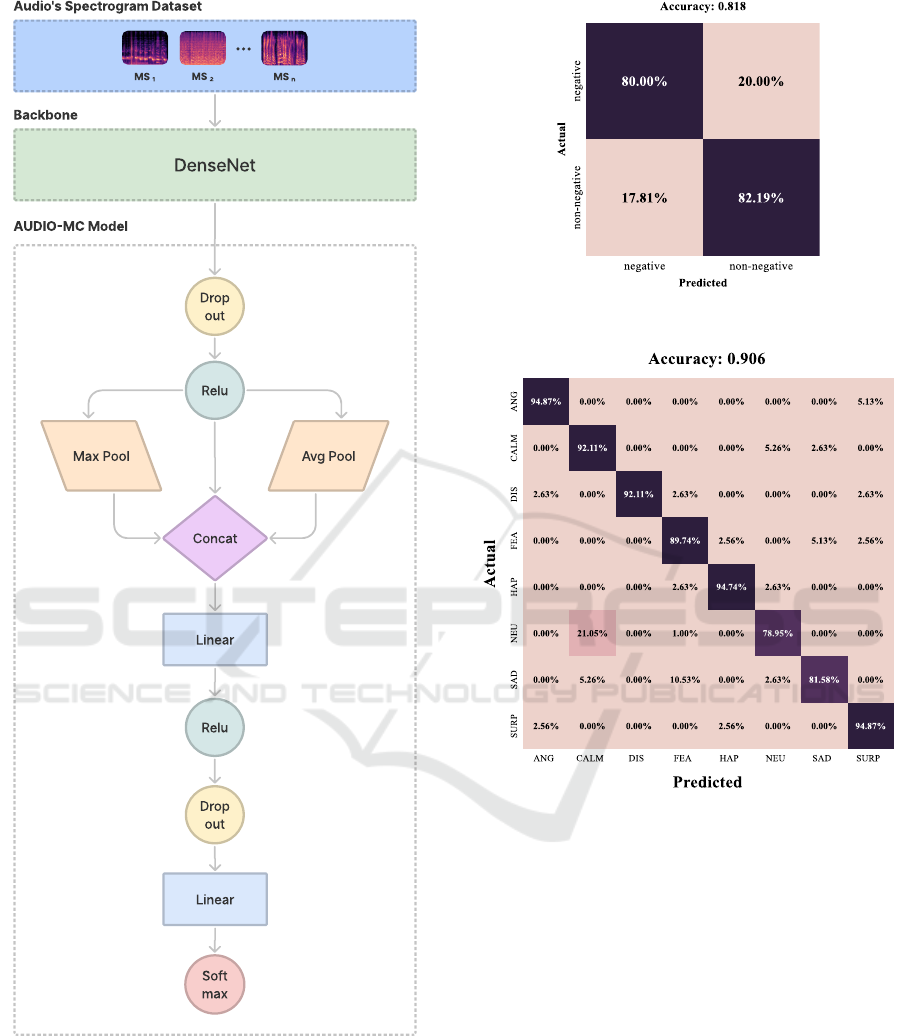
Figure 2: AUDIO-MC model architecture.

Analyzing the confusion matrix illustrated in Fig-

ure 4, we can observe that AUDIO-MC achieved an

overall accuracy of over 90%. Besides, we can note

that in ﬁve classes, the accuracy is higher than 92%,

whereas, in the FEA class AUDIO-MC achieved an

accuracy of almost 90%. However, in the other two

classes remaining, NEU and SAD, the accuracy was

Figure 3: ICMA dataset confusion matrix.

Figure 4: RAVDESS dataset confusion matrix.

around 80%. Analyzing these two classes separately:

it is essential to highlight that the SAD’s mispre-

diction occurred in a scattered way among the other

classes. At the same time, in the NEU, the prediction

error was concentrated in the CALM class, which in-

dicates that AUDIO-MC could not capture the char-

acteristics that distinguish the audios of these two

classes.

Figure 5 presents the confusion matrix and the

accuracy value for AUDIO-MC using the SAVEE

dataset. We can note that AUDIO-MC achieved

around 80% overall accuracy. Even though both

datasets have the same classes, it is already possi-

ble to observe that AUDIO-MC presents more difﬁ-

culty in classifying the audios of the SAVEE dataset

than the RAVDESS dataset. As we can see, in only

three classes, the AUDIO-MC achieved an accuracy

ICEIS 2022 - 24th International Conference on Enterprise Information Systems

380

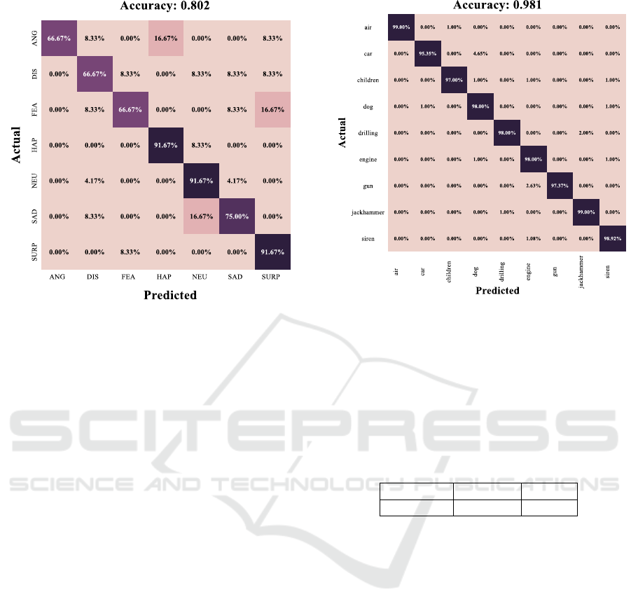
Figure 5: SAVEE dataset confusion matrix.

of more than 90%, which are: HAP, NEU, and SURP.

In the other classes, AUDIO-MC always confuses the

correct class with another class, with an error of ap-

proximately 17%. The only exception is the DIS

class, where the error is spread across several other

classes by AUDIO-MC. In fact, in Section 5.4 we

compare the result of our model with the state-of-the-

art ones, and we notice that the SAVEE dataset is ac-

tually more problematic than RAVDESS dataset. So,

AUDIO-MC achieved a still reliable result. Consider-

ing that AUDIO-MC managed to overcome more than

80% global accuracy in emotion recognition, we con-

cluded that it is also very reliable for this context.

5.3 Case Study 3: Environmental Sound

Classiﬁcation

To evaluate the AUDIO-MC performance in the con-

text of emotion recognition, we explored two datasets:

UrbanSound8k and ESC-50. Figure 6 presents the

confusion matrix and the accuracy value for AUDIO-

MC using the UrbanSound8k dataset.

Analyzing the confusion matrix illustrated in Fig-

ure 6, we can observe that AUDIO-MC had an ex-

citing result for all classes, achieving an astounding

overall accuracy of approximately 98%. This result

is related to the characteristic of the audios present in

the UrbanSound8k dataset. As the audios are pretty

distinct, AUDIO-MC can capture all the details that

differentiate them and, consequently, make a reason-

able classiﬁcation. AUDIO-MC achieved an accuracy

of over 97% across all classes. Nevertheless, it is es-

sential to point out that AUDIO-MC only achieved

Figure 6: URBAN dataset confusion matrix.

this result after tuning the hyperparameters through

Bayesian optimization.

The ESC-50 dataset is composed of audios clas-

siﬁed into ﬁfty classes. Due to a large number of

classes, we chose to present the Accuracy, F1-score

and ROC metrics instead of presenting the confusion

matrix. Table 3 presents these metrics.

Table 3: Accuracy, F1-score and ROC of ESC-50’s result.

Accuracy F1-score ROC

0.9321 0.8922 0.9656

In the ESC-50 dataset, AUDIO-MC achieved an

overall accuracy of approximately 93%. Furthermore,

to ensure no bias concern, we also have that the F1-

score and ROC were 0.8922 and 0.9656, respectively.

Therefore, the accuracy of the individual classes is

also balanced, which ensures that AUDIO-MC is a

reliable predictor for the ESC-50. For all exposed,

we conclude that AUDIO-MC framework is also ade-

quate to classify environmental sound.

5.4 Overall Comparison

We also compare the AUDIO-MC with ﬁve state-of-

the-art specif approaches. Table 4 summarizes the ac-

curacy values achieved by these approaches for each

explored dataset.

First, it is essential to highlight that we did not ﬁnd

any similar approach for audio sentiment analysis or

even a public dataset. So, we do not have a competitor

for ICMA dataset. However, we presented at least two

related works for the other four datasets.

AUDIO-MC: A General Framework for Multi-context Audio Classiﬁcation

381

Table 4: AUDIO-MC and the main related works accuracy results.

Work/dataset ICMA ESC-50 RAVDESS SAVEE URBAN

(Palanisamy et al., 2020) - 92.89% - - 87.42%

(Mushtaq and Su, 2020) - 89.28% - - 95.37%

(Kong et al., 2020) - 94.70% 72.10% - -

(Farooq et al., 2020) - - 81.30% 82.10% -

(Seo and Kim, 2020) - - 83.33% 75.00% -

AUDIO-MC 81.80% 93.21% 90.60% 80.20% 98.10%

In the emotion recognition context, the AUDIO-

MC presented the best result for the RAVDESS

dataset, improving the accuracy by approximately

8% regarding the state-of-the-art best result (Seo and

Kim, 2020). On the other hand, in the SAVEE dataset,

the AUDIO-MC showed a slight accuracy deteriora-

tion of less than 2.4%, resulting in a slight loss com-

pared to the result achieved by (Farooq et al., 2020).

In any case, we can argue that AUDIO-MC is very

competitive with the state-of-the-art in the emotion

recognition context.

In the environmental sound classiﬁcation context,

the AUDIO-MC presented an accuracy quite close

to that achieved by (Kong et al., 2020) for ESC-50

dataset. More precisely, the accuracy of AUDIO-MC

is only 1.5% less than the state-of-the-art best result.

Besides, the AUDIO-MC showed the best result for

the Urban dataset, improving the accuracy by approx-

imately 3% regarding the state-of-the-art best result

(Mushtaq and Su, 2020). Consequently, AUDIO-MC

is also competitive with state-of-the-art models for

classifying environmental sounds. Finally, we can

argue that the AUDIO-MC is generic enough to be

competitive in several contexts with state-of-the-art

models, particularly in sentiment analysis, emotion

recognition and environmental sound classiﬁcation,

as shown by the experimental results.

6 CONCLUSION

In this work, we proposed a multi-context frame-

work for audio classiﬁcation called AUDIO-MC. The

main goal of AUDIO-MC is to make more accessible

the development of audio classiﬁers supporting ma-

chine learning practitioners without professional au-

dio analysis knowledge. The AUDIO-MC performed

as well as the state-of-the-art in the most common

public audio datasets available, such as ESC-50, UR-

BAN, RAVDESS, and SAVEE. The experimental re-

sults also pointed out AUDIO-MC performed as well

as the state-of-the-art in the three different analyzed

contexts. In the sentiment analysis context, AUDIO-

MC achieved an accuracy of 81.80% on the ICMA

dataset. In the context of SER, AUDIO-MC achieved

an accuracy of 90.60% and 80.20% on RAVDESS

and SAVEE datasets, respectively. In the environ-

ment sound classiﬁcation, AUDIO-MC achieved an

accuracy of 93.21% and 98.10% on ESC-50 and UR-

BAN datasets, respectively. Besides, the AUDIO-MC

framework overcomes the state-of-the-art specif ap-

proaches on RAVDESS and URBAN datasets. As fu-

ture work we intent to extend the AUDIO-MC frame-

work using a multi-language approach.

ACKNOWLEDGMENTS

This work was partially funded by Lenovo, as

part of its R&D investment under Brazil’s In-

formatics Law, CAPES/Brazil (under grant num-

bers 88887.609129/2021, 88882.454568/2019-01,

88882.454584/2019-01 and 88881.189723/2018-01)

and LSBD/UFC.

REFERENCES

Badr., Y., Mukherjee., P., and Thumati., S. (2021). Speech

emotion recognition using mfcc and hybrid neural net-

works. In Proceedings of the 13th International Joint

Conference on Computational Intelligence - NCTA,,

pages 366–373. INSTICC, SciTePress.

Bleiweiss, A. (2020). Predicting a song title from audio em-

beddings on a pretrained image-captioning network.

In ICAART (2), pages 483–493.

Collobert, R., Weston, J., Bottou, L., Karlen, M.,

Kavukcuoglu, K., and Kuksa, P. P. (2011). Natural

language processing (almost) from scratch. J. Mach.

Learn. Res., 12:2493–2537.

de Jong, J. (2021). Signal-processing of audio for speech-

recognition. Bachelor’s thesis, Delft University of

Technology.

Facebook (2019). Adaptive experimentation platform.

https://ax.dev/. Accessed: 2021-11-15.

Farooq, M., Hussain, F., Baloch, N. K., Raja, F. R., Yu, H.,

and Zikria, Y. B. (2020). Impact of feature selection

algorithm on speech emotion recognition using deep

convolutional neural network. Sensors, 20(21):6008.

Feng, P., Lin, Y., Guan, J., Dong, Y., He, G., Xia, Z., and

Shi, H. (2019). Embranchment cnn based local cli-

mate zone classiﬁcation using sar and multispectral

ICEIS 2022 - 24th International Conference on Enterprise Information Systems

382

remote sensing data. In IGARSS 2019-2019 IEEE In-

ternational Geoscience and Remote Sensing Sympo-

sium, pages 6344–6347. IEEE.

Gorbova, J., Lusi, I., Litvin, A., and Anbarjafari, G. (2017).

Automated screening of job candidate based on mul-

timodal video processing. In Proceedings of the IEEE

conference on computer vision and pattern recogni-

tion workshops, pages 29–35.

Huang, G., Liu, Z., Van Der Maaten, L., and Weinberger,

K. Q. (2017). Densely connected convolutional net-

works. In Proceedings of the IEEE conference on

computer vision and pattern recognition, pages 4700–

4708.

Huang, G., Liu, Z., and Weinberger, K. Q. (2016).

Densely connected convolutional networks. CoRR,

abs/1608.06993.

Jackson, P. and Haq, S. (2014). Surrey audio-visual ex-

pressed emotion (savee) database. University of Sur-

rey: Guildford, UK.

Kingma, D. P. and Ba, J. (2014). Adam: A

method for stochastic optimization. arXiv preprint

arXiv:1412.6980.

Kong, Q., Cao, Y., Iqbal, T., Wang, Y., Wang, W., and

Plumbley, M. D. (2020). Panns: Large-scale pre-

trained audio neural networks for audio pattern recog-

nition. IEEE ACM Trans. Audio Speech Lang. Pro-

cess., 28:2880–2894.

Kopparapu, S. K. (2015). Non-linguistic analysis of call

center conversations. Springer.

LeCun, Y., Bottou, L., Bengio, Y., and Haffner, P. (1998).

Gradient-based learning applied to document recogni-

tion. Proceedings of the IEEE, 86(11):2278–2324.

Livingstone, S. R. and Russo, F. A. (2018). The ryerson

audio-visual database of emotional speech and song

(ravdess): A dynamic, multimodal set of facial and

vocal expressions in north american english. PloS one,

13(5):e0196391.

Lu, H., Zhang, H., and Nayak, A. (2020a). A deep neural

network for audio classiﬁcation with a classiﬁer atten-

tion mechanism. arXiv preprint arXiv:2006.09815.

Lu, L. and Hanjalic, A. (2009). Audio Classiﬁcation, pages

148–154. Springer US, Boston, MA.

Lu, Q., Li, Y., Qin, Z., Liu, X., and Xie, Y. (2020b).

Speech recognition using efﬁcientnet. In Proceedings

of the 2020 5th International Conference on Multime-

dia Systems and Signal Processing, pages 64–68.

Mushtaq, Z. and Su, S.-F. (2020). Environmental sound

classiﬁcation using a regularized deep convolutional

neural network with data augmentation. Applied

Acoustics, 167:107389.

Mustaqeem, Sajjad, M., and Kwon, S. (2020). Clustering-

based speech emotion recognition by incorporating

learned features and deep bilstm. IEEE Access,

8:79861–79875.

Noroozi, F., Marjanovic, M., Njegus, A., Escalera, S., and

Anbarjafari, G. (2017). Audio-visual emotion recog-

nition in video clips. IEEE Transactions on Affective

Computing, 10(1):60–75.

Palanisamy, K., Singhania, D., and Yao, A. (2020). Re-

thinking CNN models for audio classiﬁcation. CoRR,

abs/2007.11154.

Paszke, A., Gross, S., Chintala, S., Chanan, G., Yang, E.,

DeVito, Z., Lin, Z., Desmaison, A., Antiga, L., and

Lerer, A. (2017). Automatic differentiation in pytorch.

NIPS Workshop.

Piczak, K. J. (2015). ESC: dataset for environmental sound

classiﬁcation. In Zhou, X., Smeaton, A. F., Tian, Q.,

Bulterman, D. C. A., Shen, H. T., Mayer-Patel, K., and

Yan, S., editors, Proceedings of the 23rd Annual ACM

Conference on Multimedia Conference, MM ’15, Bris-

bane, Australia, October 26 - 30, 2015, pages 1015–

1018. ACM.

Salamon, J., Jacoby, C., and Bello, J. P. (2014). A dataset

and taxonomy for urban sound research. In Hua,

K. A., Rui, Y., Steinmetz, R., Hanjalic, A., Natsev,

A., and Zhu, W., editors, Proceedings of the ACM In-

ternational Conference on Multimedia, MM ’14, Or-

lando, FL, USA, November 03 - 07, 2014, pages 1041–

1044. ACM.

Seo, M. and Kim, M. (2020). Fusing visual attention CNN

and bag of visual words for cross-corpus speech emo-

tion recognition. Sensors, 20(19):5559.

Thornton, B. (2019). Audio recognition using mel spectro-

grams and convolution neural networks.

Uc¸ar, M. K., Bozkurt, M. R., and Bilgin, C. (2017). Signal

processing and communications applications confer-

ence. IEEE.

Van Uden, C. E. (2019). Comparing brain-like represen-

tations learned by vanilla, residual, and recurrent cnn

architectures. Phd thesis, Dartmouth College.

Xu, Y., Kong, Q., Wang, W., and Plumbley, M. D. (2018).

Large-scale weakly supervised audio classiﬁcation us-

ing gated convolutional neural network. In 2018 IEEE

international conference on acoustics, speech and sig-

nal processing (ICASSP), pages 121–125. IEEE.

AUDIO-MC: A General Framework for Multi-context Audio Classiﬁcation

383